
Contribution-Factor based Fuzzy Min-Max Neural Network: Order-Dependent Clustering for Fuzzy System Identification
- DOI
- 10.2991/ijcis.11.1.57How to use a DOI?
- Keywords
- fuzzy min-max neural network; clustering; adaptive resonance theory; contribution-factor; order-dependent; fuzzy inference system
- Abstract
This study addresses the construction of Takagi-Sugeno-Kang (TSK) fuzzy models by means of clustering. A contribution-factor based fuzzy min-max neural network (CFMN) is developed based on Simpson’s well-known fuzzy min-max neural network (FMNN) for clustering. The contribution-factor (CF) is also known as the typical pattern, and the membership threshold above which a pattern can be a CF of a cluster can be specified by the user. The stability issue is addressed and unnecessary overlaps in FMNN can be avoided. Furthermore, two considerations are combined in the clustering process to fully exploit the information in the data: 1) patterns (points) are generated in a sequence, so it’s reasonable to capture the order-dependent information of data, and 2) the clustering process shouldn’t be influenced too much by noisy data or outliers. As a result, CFMN can put most cluster centers in high-density regions of clusters without influence of the low-density regions. This feature is very important when clusters are used as fuzzy rules because the high-density region of some cluster can be interpreted as the most common part of that rule. Simulations are performed to illustrate the clustering behavior of CFMN and identification performance of the resulting fuzzy inference system (CFMN-FIS). It is shown that the proposed algorithm is fast to learn and has good prediction performance.
- Copyright
- © 2018, the Authors. Published by Atlantis Press.
- Open Access
- This is an open access article under the CC BY-NC license (http://creativecommons.org/licences/by-nc/4.0/).
1. Introduction
Fuzzy identification is an effective tool for the approximation of uncertain nonlinear systems on the basis of measured data. The data driven construction of fuzzy models has become an important topic of research with a wide range of real-world applications. The Takagi-Sugeno-Kang (TSK)1 model is a method of fuzzy inference well known in the fuzzy systems literature. The great advantage of the TSK model is its representative power. It is capable of describing a highly nonlinear system using a small number of rules2. Generally, fuzzy system identification consists of structure identification and parameter learning. Structure identification is used to determine the fuzzy membership functions and the appropriate number of rules. Parameter learning concerns the calculation of coefficients of each rule. As to the TSK model, the structure identification is based on a fuzzy partition of the input space and the parameter learning can be performed by standard linear least-squares methods when the premise parameters are fixed.
One of the most common approaches to structure identification is the utilization of clustering analysis. As defined in Ref. 3, the goal of clustering analysis is to discover natural groups of a set of points according to intrinsic characteristics or similarity. In other words, clustering divides data into groups, in such a manner that similar instances are grouped in the same group, producing a concise representation of a system’s behavior4. Moreover, groups can be used to establish some hypothesis about the structure present in the data. Compared with other classical methods of membership functions identification that are complex or computationally demanding, for example, gradient descent5, genetic algorithms6, and Kalman filtering7, clustering can be used to make groups of related data and reduce the complexity of the model when we have a lot of data and we have no more information about it8.
Although many clustering algorithms have been used for fuzzy modeling491011, there are two considerations that have not been combined to fully exploit the information in the data.
- 1.
Most of the clustering algorithms proposed in the literature didn’t consider the order-dependent information. As the patterns (points) are generated by the underlying system in a sequence, not in a bunch, it’s reasonable to capture the order-dependent information of data. In fuzzy system identification, the rule can be seen as a cluster in the feature space, thus if the clusters can adapt according to the information accounting for pattern generation order, we will get more informative rules.
- 2.
Uncertainty in the data should be considered. That is, the clustering process shouldn’t be influenced too much by noisy data or outliers.
This motivates us to use the fuzzy min-max clustering neural network (FMNN)12 with conceptually simple but powerful on-line learning process13. The network is order-dependent in the sense that the clustering result may be different if the input patterns are presented to the algorithm in a different order. However, FMNN doesn’t consider the noise contained in patterns and tries to include all patterns in hyperboxes (clusters). This makes the network very unstable and the clusters generated are very close to each other.
In this paper, the contribution-factor based fuzzy min-max neural network (CFMN) is developed based on FMNN to explicitly exploit the order-dependent information in the clustering process and incorporates significant modifications that improve the noise-resistant capability of FMNN. The contribution-factor (CF) is also known as the typical pattern, and the membership threshold above which a pattern can be a CF of a cluster can be specified by the user. CFMN also introduces a parameter that specifies the minimum inter-cluster distance to ensure well-separated clusters. Furthermore, CFMN can put most cluster centers in the high-density region of clusters without influence of low-density regions. This feature is very important when clusters are used as fuzzy rules because the high-density region of some cluster can be interpreted as the most common part of that rule. Performance of the resulting fuzzy inference system (CFMN-FIS) is demonstrated on two nonlinear benchmark processes and three real-world data sets widely used in the fuzzy modeling literature. The obtained results are compared with results from the literature. It is shown that the proposed algorithm is fast to learn and has good prediction performance.
The main contributions are summarized as follows:
- 1.
This study shows that the data-order information can be exploited in the clustering process. This information helps to discover the high-density region of clusters.
- 2.
We find that the learning process of FMNN has some kind of periodicity, which significantly impacts on the stability performance.
- 3.
The proposed CFMN is intuitive in parameter choosing. The user can easily specify the cluster size and inter-cluster distance according to different situations.
- 4.
CFMN has two advantages over existing clustering algorithms. Firstly, the estimated clusters are not affected by the clusters which the algorithm fails to discover. Secondly, the high-density region of a cluster is enclosed by a hyperbox without influence of low-density regions. These two features are essential to generate more meaningful fuzzy rules for the TSK-type CFMN-FIS.
The rest of this paper is organized as follows. Section 2 analyses the stability issue of FMNN. In Section 3, a detailed description of CFMN is given. Section 4 describes the resulting fuzzy model. Section 5 illustrates the feature of CFMN. The comparison of CFMN-FIS with various algorithms are also given. Finally, conclusions are given in Section 6.
2. Analysis of FMNN
This section will review the essential concepts of FMNN, and discuss its stability issue. The proposed CFMN will be introduced in Section 3.
The fuzzy min-max clustering neural network (FMNN)12 is constructed by using hyperbox fuzzy sets. A hyperbox is completely defined by its min point and max point. The combination of the minmax points and the hyperbox membership function defines a fuzzy set (cluster). Once the FMNN is trained, it is operated by presenting a pattern and computing the membership value in each of the existing fuzzy sets. Although the learning portion of the algorithm is not neural, the recall operation fits immediately into a neural network framework.
2.1. Fuzzy Hyperbox Membership Function
Let the jth hyperbox fuzzy set Bj, be defined by the ordered set
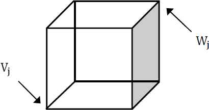
The min-max hyperbox Bj = {Vj, Wj} in ℝ3.
The membership function is defined as
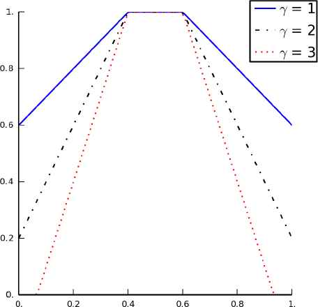
Membership function bj(Ah) of FMNN.
The membership function in FMNN measures the degree to which the hth input pattern Ah falls within the hyperbox Bj formed by the min point Vj and max point Wj. On a dimension-by-dimension basis, this can be considered a measurement of how far each component is greater than the max point value or less than the min point value12. As Ah approaches the hyperbox, bj(Ah) approaches 1. When the point is contained within the hyperbox, bj(Ah) is equal to 1.
2.2. Recasting FMNN in the Framework of ART
As a competitive learning based clustering method, FMNN has much similarity with adaptive resonance theory (ART)14. ART is a family of neural networks that develop stable recognition categories (clusters) by self-organization in response to arbitrary sequences of input patterns15. At the training stage, the stored prototype of a category (cluster) is adapted when an input pattern is sufficiently similar to the prototype. An input pattern is said to be novel to the neural network if it deviates too much from all existing prototypes, then the ART adaptively and autonomously creates a new category with the input pattern as the prototype16. An ART system relies on novelty to distinguish between familiar and unfamiliar events (patterns), as well as between expected and unexpected events17. FMNN follows the same learning paradigm except that the prototypes are represented by min-max points.
In fact, FMNN grows out of the fuzzification of the ART-1 neural network17. Here, for ease of understanding and analysis, we summarize FMNN as a three-layer network in the framework of ART171815.
The architecture is shown in Fig. 3. The input layer F0 receives and stores the input pattern. The comparison layer F1 stores the normalized input pattern also called the short-term memory. The recognition layer F2 stores the prototypes (min points and max points) of recognition categories (clusters) as the long-term memory. Learning of the FMNN consists of creating and adjusting hyperboxes in the F2 layer, trying to include all patterns in hyperboxes, and is summarized as follows.
- 1.
Parameters
The FMNN is determined by the hyperbox size constraint parameter θ, and the parameter γ controlling the fuzziness of the membership function which is usually set to 4.
- 2.
Network Initialization
The F2 layer is initialized as the null set.
- 3.
Input Normalization
The input pattern in the F0 layer is normalized from ℝn to 𝕀n, and is fed into the F1 layer.
- 4.
Category Choice
Given a pattern Ah in the F1 layer, the hyper-box Bj in the F2 layer that provides the highest degree of membership and allows expansion is identified. The expansion criterion of FMNN is
It defines the constraint regulating the average size of the hyperbox. The parameter θ (0 < θ < 1) is a user-defined value directly related to the number of hyperboxes generated in the F2 layer and significantly affects the effectiveness of the training algorithm. - 5.
Resonance or Reset
Mismatch reset happens when one of the following cases is met:
- •
Case 1: the first pattern is presented.
- •
Case 2: all existing Bj are exhausted without any expansions.
Then a new category (cluster) Bj is created by copying Ah as its min point and max point, i.e.,
Otherwise the network is said to reach resonance at hyperbox (category) Bj found in step 4), and the learning begins. - •
- 6.
Learning
The hyperbox Bj is updated according to
- 7.
Hyperbox Overlap Test
This procedure is performed immediately after the previous expansion step. Suppose that Bj is expanded, then each dimension of Bj is compared with the remaining Bk. The expansion creates an overlap between Bj and Bk if there is some kind of overlap for each of the n dimensions.
- •
Case 1: vji < vki < ωji < ωki.
- •
Case 2: vki < vji < ωki < ωji.
- •
Case 3: vji < vki ⩽ ωki < ωji.
- •
Case 4: vki < vji ⩽ ωji < ωki.
Note that the above four cases summarized in Ref. 12 are not complete, and there are four neglected boundary cases which may lead to failure of overlap test, so we restate here with corrections:
- •
Case 1: vji < vki < ωji < ωki.
- •
Case 2: vki < vji < ωki < ωji.
- •
Case 3: vji ⩽ vki ⩽ ωki ⩽ ωji.
- •
Case 4: vki ⩽ vji ⩽ ωji ⩽ ωki.
Each of these cases is illustrated in Fig. 4. The added boundary cases are illustrated by the bottom portions of Fig. 4c and Fig. 4d.
- •
- 8.
Hyperbox Contraction
The overlap between hyperbox Bj and Bk is eliminated on a dimension-by-dimension basis. Using the four cases described previously, the overlapping hyperboxes are contracted as follows to eliminate overlap in every dimension so that the resulting clusters are more compact.
- •
Case 1: If vji < vki < ωji < ωki,
- •
Case 2: If vki < vji < ωki < ωji,
- •
Case 3: If vji ⩽ vki ⩽ ωki ⩽ ωji, then the contraction is performed on the smaller of the two overlaps. If ωki − vji < ωji − vki then contract using the assignment
otherwise use the assignment - •
Case 4: If vki ⩽ vji ⩽ ωji ⩽ ωki, then, by symmetry, the same assignments under the same conditions in case 3 are applied here.
- •
- 9.
Cluster Stability Test
Steps 3)–8) are repeated for each pattern in the data set until cluster stability is achieved. Cluster stability is defined as all hyperbox min and max points not changing during successive presentations of the dataset in the same order.
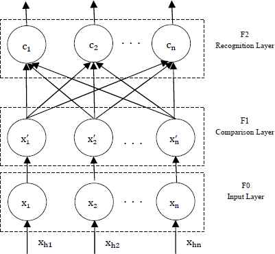
Architecture of FMNN.
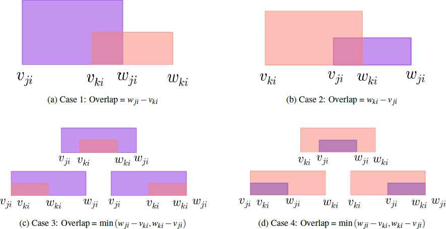
The four cases that occur during overlap testing. Each graph shows the relative values of two hyper-boxes along one dimension. Part of this figure is adapted from FMNN.
Please note that steps 4)–6) together corresponds to the hyperbox expansion procedure of the original FMNN.
2.3. The Stability Issue of FMNN
In FMNN, the inappropriate setting of θ and the randomness present in the dataset may slow down the learning algorithm and even prevent it from convergence. This is because that the expansion for patterns with low membership degree makes the clusters easy to grow up to full size, resulting in overlaps between clusters. The situation would become much more worse when many points are at the cluster boundary.
After exploring the algorithm for different parameters and datasets, we find an interesting phenomenon that the prototypes generated will reappear after every p (p ⩾ 1) presentations of the data set in step 9) of the training process, i.e., the overlap contraction process has some kind of periodicity. At the beginning of the next presentation of the dataset (represented by D), the cluster learning algorithm is based on the result of the last presentation. Hence the clusters eventually resulted are based on the dataset [D, D,···, D] of length p, not D if p > 1, and thus the clusters are not well-defined.
The above stability issue can be explained by the well-known stability-plasticity dilemma17 in the ART literature. Simply speaking, a system must have plasticity to learn about significant new events, and it must also remain stable in response to irrelevant or often repeated events. In Ref. 19, two types of stability condition named as stable1 and stable2 are defined for incremental clustering algorithms:
- 1.
stable1: No prototype vector can ”cycle”, or take on a value that it had at a previous time.
- 2.
stable2: Only a finite number of clusters are formed with infinite presentation of the data set.
FMNN fails to meet stable1 because FMNN tries to include all patterns in hyperboxes which makes the neural network too plastic.
Since we will employ the clustering neural network to generate rules for fuzzy influence system, the clustering algorithm should overcome the stability-plasticity dilemma and converge quickly. More importantly, noisy data from real world would lead to serious stability issue.
Previous discussion suggests that FMNN should be modified, so that the neural network can overcome the stability-plasticity dilemma and still performs well under noisy environment. Therefore, we introduce a new FMNN named contribution-factor based fuzzy min-max neural network (CFMN), which achieves more stability by restricting the plasticity and is more robust.
3. Proposed CFMN Clustering Algorithm
A common feature of incremental clustering algorithms is that the resulting clusters would be different if the presentation order of the data set changes. This feature will be utilized in CFMN to capture the high-density region of a cluster when the cluster is corrupted by noise. Moreover, the algorithm’s plasticity will be restricted to overcome the stability-plasticity dilemma.
3.1. Overview of CFMN
The main characteristics of CFMN are summarized as follows:
- •
The parameters are intuitive to choose.
- •
As clustering is exploratory in nature, it’s often the case that the algorithm estimates the wrong number of clusters. CFMN can ensure that the estimated cluster centers are around the real ones when the parameters are set over an appropriate range, i.e., the estimated clusters are not affected by the clusters which the algorithm fails to discover.
- •
CFMN exploits the order-dependent feature of incremental clustering to make the algorithm order-independent, i.e., the hyperboxes are designed to enclose the high-density regions of clusters, and this holds even when the data set is shuffled.
The architecture of CFMN is shown in Fig. 5. Compared with FMNN, CFMN makes the mismatch reset condition explicit and has two operation modes, i.e., normal mode and relearning mode.
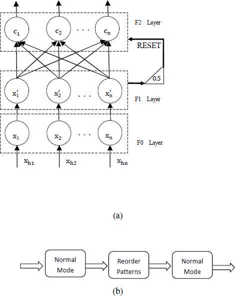
Architecture of CFMN. (a) Normal mode. (b) Relearning mode.
CFMN works in normal mode if data are generated and provided in sequence. This mode is based on the observation that data sets generated in real world represent some behavior of the underlying system and, patterns are often not equally affected by noise. Furthermore, normal (or typical) patterns are more likely to be generated first and are also more likely to form high-density regions. In contrast, patterns affected too much by noise (noisy patterns) often form the low-density region of a cluster. More specifically, each cluster is assumed to consist of one high-density region and one or several low-density regions, and CFMN aims to enclose typical patterns in hyperboxes without influence of low-density regions.
The relearning mode is chosen if the data set loses the order information. As the patterns presented first to the algorithm are closely connected to the resulting clusters, CFMN introduces the relearning mechanism to eliminate the impact of presentation order.
The development of CFMN has considered the following requirements.
- 1.
The hyperbox should only expand typical patterns.
Hyperbox expansion is an important step in the learning algorithm and it is closely related to coping with noisy patterns. Suppose that the high-density region of a cluster is first presented to the algorithm so that a hyperbox has been created for that region. Then it’s reasonable to consider patterns with low membership degree to existing clusters as noisy data. An example is shown in Fig. 6. Pattern Ah is presented to the network before A′h. We can see that Ah is closer to the hyperbox B2 than B1. However, B2 can’t meet the expansion criterion. Furthermore, Ah contains too much noise to be expanded for B1. In contrast, A′h can be seen as a typical pattern for B1 and can be expanded. Ah is neglected and doesn’t contribute to the expansion of any hyperboxes in CFMN, whereas in FMNN, Ah can be included into B1, which makes the hyperbox grow to full size quickly and the expansion sensitive to noisy patterns.
- 2.
The membership function should reflect the noise degree of a pattern.
The membership function of FMNN shown in Fig. 2 is calculated based on the pattern’s distance to the cluster boundary, i.e., bj(Ah) is close to 1 if Ah is close to the min point or max point. Then a pattern far from the cluster center can have high membership to the cluster. The authors of DCFMNN20 pointed out that the noisy data near the boundary should also be taken care of. The boundary-based membership function is widely used in the fuzzy min-max neural network literature. However, the membership degree changes dramatically with the boundary as the cluster expands. This fact suggests that it’s difficult to use the boundary-based membership function as an indicator to detect noisy data. For example, the noise level is first estimated from data in DCFMNN20. Then, bj(Ah) of the pattern Ah near the boundary is lower if the noise level is high.
As stated previously in 1), the cluster center has been supposed to lie in the high-density region. The pattern far from the cluster center often lie in the low-density region, so the data near the cluster boundary should also have low membership degree. This is achieved by implementing an exponential membership function, which makes it easier for CFMN to copy with noisy data and the detection of outliers.
- 3.
The resulting clusters should be well-separated.
Choosing parameters in FMNN lacks intuition and the generated hyperboxes are not always well-separated. This can be seen in Fig. 7a. CFMN introduces a parameter to control the inter-cluster distance. The clusters in Fig. 7b is more well-separated than in Fig. 7a. Fig. 7 also shows that the overlaps can be avoided in CFMN.
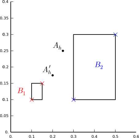
Expansion of patterns. In CFMN, Ah is neglected and only A′h can be expanded to B1.
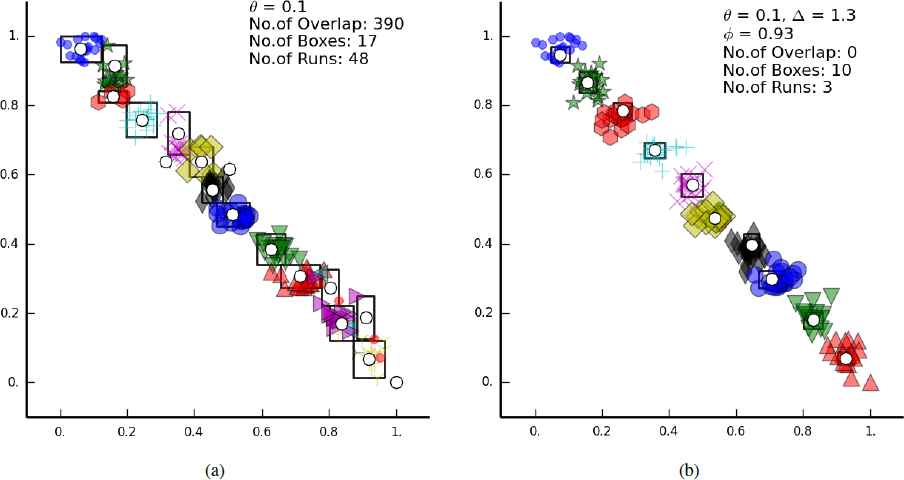
Comparison of FMNN and CFMN on a data set with 10 clusters provided in sequence. The center of each cluster is presented first. (a) Result of FMNN. (b) Result of CFMN.
3.2. Basic Definitions
In the following, we will describe the concepts of novelty, virtual boundary, and typical pattern respectively, which are essential in the development of CFMN.
Let Ah1 and Ah2 denote the input patterns, ci and cj denote the cluster centers of clusters Bi and Bj, and Vj and Wj denote the min-max points of cluster Bj. The center cj is defined as (Vj +Wj)/2. θ, d0, d1, and d2 are parameters controlling the behavior of the network. θ specifies the maximum cluster size for each dimension in an average sense (note that parameter θ of FMNN specifies the maximum hyperbox size).
The distance between Ah1 and Ah2 is defined as
The cluster boundary in FMNN is formed by the min-max points, whereas in CFMN, the hyperbox formed by the min-max points are used to enclose only a portion of the cluster. So the virtual boundary of a cluster Bj is defined as the points that satisfy
Ah is a typical (normal) pattern to Bj if
Before proceeding, we shall introduce a parameter Δ which satisfies
Next, parameters d0, d1, and d2 will be converted so that they are related to the membership degree of a pattern and more intuitive for the user to choose.
As stated previously, the membership function should decrease with the distance between pattern Ah and the centroid of hyperbox Bj in order to make it an indicator to tell good data from noisy data or outliers. To meet the required criterion, a new membership function is defined as
The membership threshold 0.5 has similar functions as the vigilance value in ART below which a new category (cluster) is created, i.e., Ah is novel to the network if minj bj(Ah) ⩽ 0.5. As we know, the creation of new hyperboxes is closely related to the detection of outliers, i.e., we shall create a new hyperbox Bj at the distance of ∆θ. Bj is either a cluster of true patterns or a cluster of outliers, and the difference is that the density is lower in the latter case. Here we explicitly relate the membership function and the creation of new hyperboxes to θ, which makes the selection of θ easier for the user.
For the pattern Ah at the virtual boundary of hyperbox Bj, we can get its membership degree from (14), (16), and (18)
In CFMN, only patterns with high membership degree (i.e., typical patterns) are allowed to contribute to the adjustment of a hyperbox. To emphasize this characteristic, a typical pattern of cluster Bj is also called a contribution-factor (CF) to Bj. In fact, CFMN introduces CF to limit the network’s plasticity, i.e., only the CF (with strong influence to some neuron) can be turned into long-term memory, thus overcoming the stability-plasticity dilemma.
3.3. CFMN in Normal Mode
The two learning modes will be introduced separately. The learning process of normal mode is similar with that of FMNN. We will only describe its main part.
- 1.
Parameters
CFMN has three parameters. θ specifies the maximum cluster size for each dimension in an average sense, Δ specifies the ratio of the minimum inter-cluster distance relative to θ, and ϕ specifies the membership threshold above which a pattern can be a CF of a cluster (ϕ ∈ (0.84,1) because a CF must lie in the virtual boundary of a cluster).
- 2.
Network Initialization
The F2 layer is initialized as the null set.
- 3.
Input Normalization
The input pattern in the F0 layer is normalized to 𝕀n, then it is fed into the F1 layer. This step is optional since the membership function is of Gaussian type.
- 4.
Category Choice
Given a pattern Ah in the F1 layer, the hyper-box Bj in the F2 layer that provides the highest degree of membership and allows expansion is identified. The expansion criterion is
It implies that the cluster Bj shouldn’t expand for Ah if Bj becomes too full after expansion, or if Ah is not a CF (typical pattern) of Bj. - 5.
Resonance or Reset
Mismatch reset happens when one of the following cases is met:
- •
Case 1: the first pattern is presented.
- •
Case 2: maxj bj(Ah) ⩽ 0.5., i.e., novelty is detected.
Then a new category (cluster) Bj is created by copying Ah as its min point and max point, i.e.,
Otherwise the network is said to reach resonance at hyperbox (category) Bj found in step 4), and the learning begins. - •
- 6.
Learning
- 7.
Hyperbox Overlap Test
- 8.
Hyperbox Contraction
Steps 6)–8) are same with that of FMNN.
- 9.
Cluster Stability Test
Steps 3)–8) are repeated for each pattern of the data set in the same order until cluster stability is achieved. Note that the stability issue encountered in FMNN may occur here when the network has large plasticity, i.e., ϕ is set around 0.84, which implies that patterns along the virtual boundary are allowed to be expanded. Increasing the value of ϕ can solve this issue and can also significantly speed up the learning process.
3.4. CFMN in Relearning Mode
Clustering algorithms such as the K-Means and Expectation Maximization, require to specify the number of clusters before the clustering process. In contract, FMNN and CFMN require to specify the cluster size of individual dimension. Just as K-Means and Expectation Maximization that are sensitive to the initialization of cluster centers, the order of input patterns during training affects the nodes (clusters) in the F2 layer of CFMN or FMNN, which is a common feature for incremental learning algorithms. The common method to solve this problem is to present training patterns in random order, where voting strategy is used to compute the final performance. Genetic algorithm and Particle Swarm Optimization have also been used to select the presentation order of training patterns2122.
As stated previously, the presentation order is utilized in normal mode of CFMN to capture the high-density region of a cluster when the cluster is corrupted by noise and the data set is provided in sequence. However, the high-density region can’t be captured perfectly when the data set loses the order information, which is often the case.
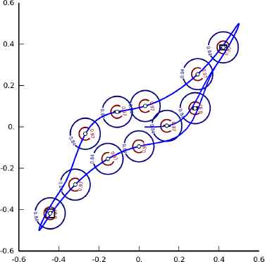
The introduction of CF can limit the plasticity of the network, i.e., a hyperbox can only expand near patterns, and its center will not move dramatically since it’s created if the user specifies a large ϕ. The relearning mode relies on this fact to capture the high-density region. The architecture of this mode is shown in Fig. 5b. The patterns are first clustered in CFMN normal mode, then patterns in each cluster are sorted by density before applying CFMN normal mode again. In the second applying of CFMN normal mode, the high-density region of each cluster is presented first and enclosed by the hyperbox. Density estimation is performed using the kernel density estimation (KDE)23
The relearning mechanism can ensure that the resulting clusters are not affected too much by the noisy patterns. For illustration, this mode is run on the popular ruspini24 data set. The data set is shuffled before clustering. The result is shown in Fig. 8. The high-density region of each cluster is perfectly captured by the hyperbox and the cluster represented by stars in the figure can be seen as an outlier cluster.
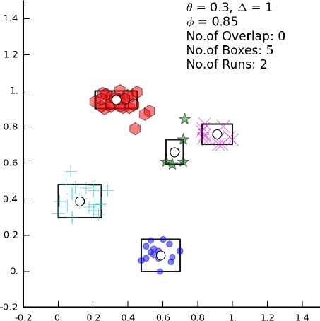
Result of CFMN on the ruspini data set. The data set is shuffled before clustering.
4. CFMN Fuzzy Inference System
The clustering algorithm has been introduced in Section 2 and Section 3. Now we will concentrate on the construction of fuzzy models.
A fuzzy system consists of a bunch of fuzzy if-then rules. Generally, fuzzy system identification consists of structure identification and parameter learning. Structure identification is used to determine the fuzzy membership functions and the appropriate number of rules. Parameter learning estimates the coefficients of each rule.
In the proposed CFMN fuzzy inference system (CFMN-FIS), the clusters generated by CFMN are used as fuzzy rules. That is, the premise parameters (membership functions of input variables) are specified by the clusters and the input parameters of CFMN. Note that CFMN works in normal mode when the data set is provided in sequence. Otherwise CFMN works in relearning mode. The resulting fuzzy system is of the following Takagi-Sugeno-Kang (TSK) form:
Rule j : IF x1 is Aj1 AND⋯AND xn is Ajn
For the jth Rule that is represented by cluster center cj (middle point of the min and max points Vj, Wj), fuzzy set Aji is given by
The fire strength µj(x) of Rule j is calculated by using multiplication as the AND operator
5. Experimental Results
Demonstration of CFMN and CFMN-FIS will now be given on a variety of data sets. The first two examples relate to clustering characteristics of CFMN and the remaining three relate to CFMN-FIS. FMNN-FIS is also constructed in the same way as CFMM-FIS for comparison.
5.1. Example 1—the Order-dependent Feature of CFMN
The data used in this example is constructed in order to illustrate the order-dependent feature of CFMN. More specifically, the estimated cluster centers are around the real ones when the parameters are set over an appropriate range, i.e., the estimated clusters are not affected by the clusters which the algorithm fails to discover. We also show that the introduction of D offers the user more control over the clustering process. This data set consists of 100 input patterns for each cluster. It’s generated by 3 Gaussian blobs which are denoted by Cluster A, B, C with standard deviation 0.3 and with centers [(1, 1), (−1, −1), (1, −1)] respectively. The true clusters are shown in Fig. 9a. We can see that the hyperbox size is approximately 2 and the inter-cluster distance 2. So the parameters of CFMN can be chosen as [θ = 2, Δ = 1, ϕ = 0.93]. Please note that the setting of ϕ here is arbitrary and the training will be fast if ϕ is large because the number of CF will be very small.
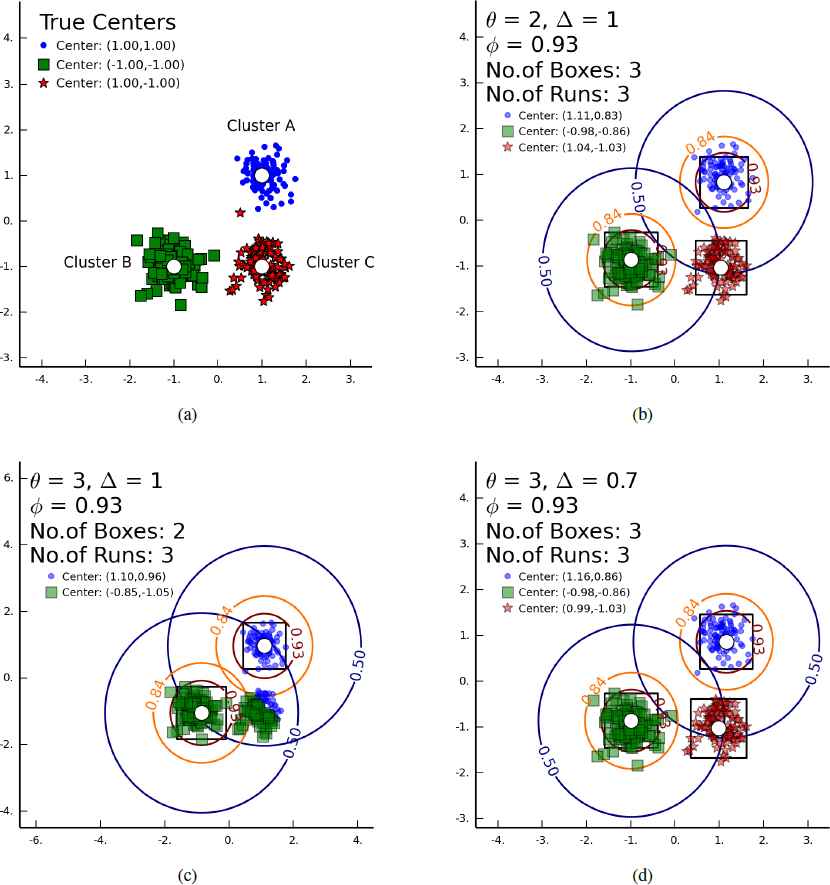
Clustering result of Example 1. The centers estimated by CFMN are represented by big circles and the hyperboxes are represented by rectangles.
To illustrate the benefit of Δ’s control over the clustering process, the training of the network for two different settings of θ has been carried out. The clusters are presented to the algorithm in the generation order: [Cluster A, Cluster B, Cluster C]. The parameters and clustering results including the estimated centers are shown in Fig. 9. Contour plots of the membership function with three levels [0.5, 0.84, 0.93] are also shown, and for clarity, only two clusters in each subfigure are plotted with contours. Note that 0.5 is a threshold to determine if the pattern is novel to the network and the virtual boundary of each cluster is represented by the membership value with level of 0.84
Fig. 9b shows the results of appropriate setting of parameters. In Fig. 9c, θ is set to 3, which is apparently too large and results in only two clusters, but it’s interesting to observe that the two estimated cluster centers are still very close to the real ones. The reason why the estimated centers of Cluster A and Cluster B are not affected by Cluster C is that in CFMN clusters evolve by expansion of CFs. The evolving stops because of the lack of CF caused by gaps between pattern regions. In Fig. 9d, the undesirable effects of large θ is fortunately avoided when we adjust Δ to 0.7. Although the clusters are almost the same in Fig. 9b and Fig. 9d, the clusters are allowed to grow a bit larger in the latter case because of larger θ.
For comparison, the results of FMNN is shown in Fig. 10. In Fig. 10a, points that belongs to Cluster C are wrongly enclosed by Cluster B. In Fig. 10b, FMNN also estimates 2 clusters when θ = 3, however, Cluster A and Cluster C are merged and the estimated cluster center is also affected by this merge.
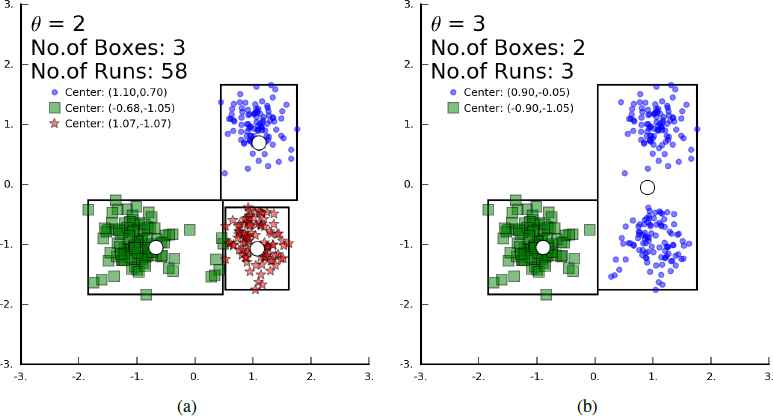
The clustering result of FMNN on dataset Fig. 9a.
This example shows that the utilization of order-dependent information enables CFMN to discover the high-density regions of clusters more robustly than FMNN. This feature also allows CFMN to generate fuzzy rules in a more reasonable way for a wider range of parameters than FMNN. In other words, the input space of the system can be more easily covered. In order to exploit the order-dependent information, CFMN also improves the noise-resistant capability, as will be seen in the next example.
5.2. Example 2—the Stability Feature and the Enhanced Error-rejection Characteristic of CFMN
This example is included to illustrate the stability feature and the enhanced error-rejection characteristic of CFMN. The stability issue of FMNN is addressed by CFMN via restricting the plasticity with parameter ϕ. More specifically, CFMN introduces the CF strategy to reduce the unnecessary overlaps in FMNN, and also gains more stability over FMNN. We reproduce the dataset of GFMM13. The original data set consists of 41 patterns, 40 of which were randomly generated around point (0.25, 0.25) within 0.05 range, and the remaining one represented an outlier. We add a small cluster of 20 patterns on the right in order to make sure that the when the algorithm’s parameters are chosen to detect outliers, the algorithm should still produce reasonable clusters. Fig. 11 illustrates the advantage of CFMN. The outlier can be detected at very large θ whereas FMNN suffers the problem at large θ. We can also see that CFMN avoids the unnecessary overlaps in FMNN. Please note that hyperbox overlaps directly reflect the plasticity of the network, and thus can indicate the stability.
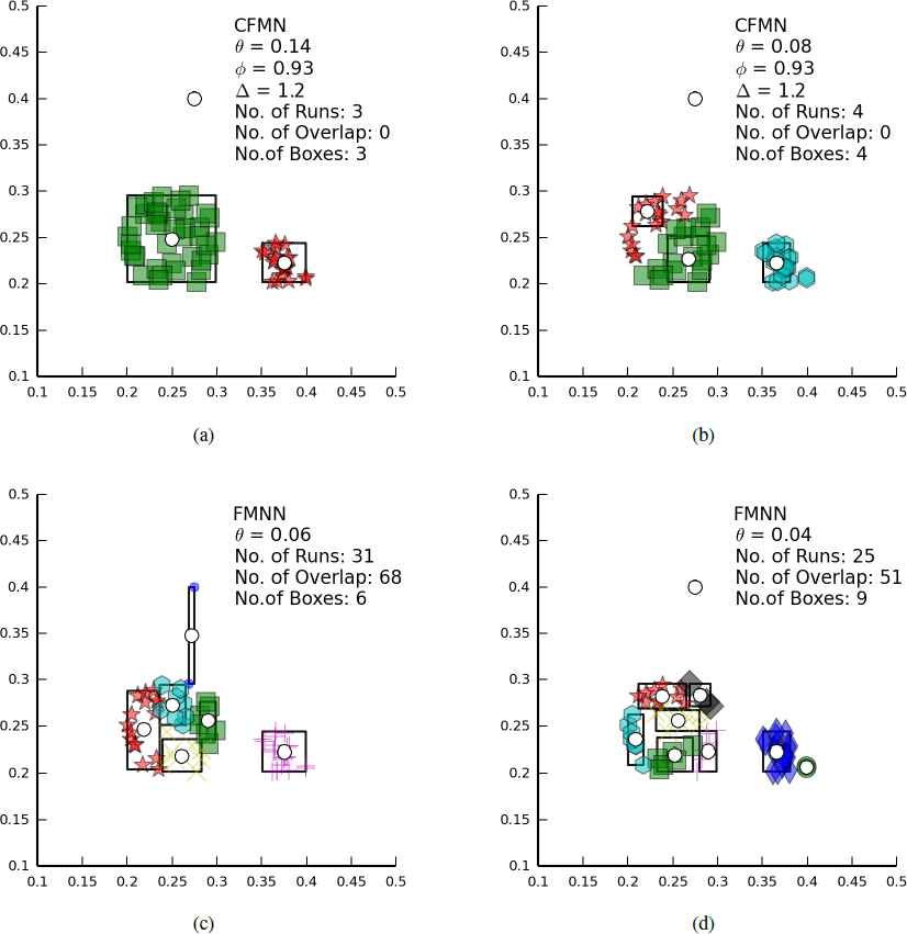
Clustering in presence of outlier.
5.3. Example 3—Identification of the Dynamic System
In this example, CFMN-FIS is used to identify a dynamic system described by Juang and Lin25.
Input space and final assignment of rules corresponding to CFMN-FISb of Example 3.
| Algorithm | Type | N | K | RMSEtrain | RMSEtest |
|---|---|---|---|---|---|
| RIT2NFS-WB | Type-2 | 200 | 7 | 0.0021 | 0.0021 |
| SEIT2FNN | Type-2 | 200 | 7 | 0.0022 | 0.0022 |
| McIT2FIS-US | Type-2 | 50000 | 5 | 0.0006 | 0.0006 |
| McFIS | Type-1 | 50000 | 20 | 0.0023 | 0.0023 |
| eTS | Type-1 | 50000 | 19 | - | 0.0080 |
| SAFIS | Type-1 | 50000 | 8 | - | 0.0112 |
| SONFIN | Type-1 | 50000 | 10 | - | 0.0130 |
| FMNN-FIS | Type-1 | 200 | 15 | 0.0024 | 0.0023 |
| FMNN-FIS | Type-1 | 50000 | 16 | 0.0013 | 0.0013 |
| CFMN-FISa | Type-1 | 200 | 6 | 0.0015 | 0.0015 |
| CFMN-FISb | 200 | 11 | 0.0007 | 0.0008 | |
| CFMN-FISc | 200 | 25 | 0.0005 | 0.0005 | |
| CFMN-FISa | 50000 | 6 | 0.0009 | 0.0009 | |
| CFMN-FISb | 50000 | 11 | 0.0001 | 0.0001 | |
| CFMN-FISc | 50000 | 25 | 0.00008 | 0.00008 | |
Performances of various fuzzy models for the dynamic system of Example 3. N represents the training size, K represents the number of rules.
From Table 1 we can see that CFMN-FIS can generalize well to a small K, and achieves state-of-the-art results on this dataset. Note that, this dataset is provided in sequence. FMNN-FIS also captures the order-dependent information. However, the performance of FMNN-FIS with training size 200 is not good as RIT2NFS-WB and SEIT2FNN. In contrast, the performance of CFMN-FIS is good in both training cases. This example shows that CFMN-FIS has good performance on datasets provided in sequence because of the utilization of order-dependent information.
5.4. Example 4—Mackey-Glass Time-Series Prediction
This example studies the prediction of the following Mackey-Glass chaotic time series:
| Algorithm | K | RMSEtrain | RMSEtest |
|---|---|---|---|
| RBF1 | - | - | 0.0013 |
| RBF2 | - | 0.0012 | 0.0013 |
| ANFIS | 16 | 0.0016 | 0.0015 |
| GEFREX | 20 | 0.0054 | 0.0061 |
| RBF-AFS | 23 | 0.0096 | 0.0114 |
| FMNN-FIS | 47 | 0.0036 | 0.0037 |
| CFMN-FISa | 36 | 0.0016 | 0.0015 |
| CFMN-FISb | 52 | 0.0012 | 0.0011 |
| CFMN-FISc | 72 | 0.0010 | 0.0009 |
Performances of various fuzzy models for mackey-glass of Example 4. K represents the number of rules. RBF1 and RBF2 are two RBF networks.
5.5. Example 5—Identification Performances on Three Real-World Data Sets
In this example, the identification performance of CFMN-FIS is tested on three real-world data sets widely used in the fuzzy modeling literature. These data sets are neither arranged in generating order, nor in bunch of clusters. The purpose of this example is to show that CFMN-FIS is still able to learn the underlying system even when the input patterns are shuffled.
The first is the Box-Jenkins furnace data set35. It consists of 296 data points [u(t), y(t)], from t = 1 to 296, where u(t) is the input gas flow rate and y(t) is the output CO2 concentration. The system is modeled by ŷ(t) = f(u(t − 4), y(t − 1)) and all the samples are used for training as done in Ref. 27. The parameters of CFMN-FIS on this data set are [θ = 0.17, ϕ = 0.96, Δ = 1]. FMNN-FIS is run with θ = 0.2.
The second is the abalone data set collected from the UCI machine learning repository. It consists of 4177 samples. The data are generated with random sampling, with 3342 samples for training and the remaining 835 samples for testing. The features length, diameter, height, whole weight, shucked weight, viscera weight, and shell weight are taken as input, the number of rings is taken as output as done in Ref. 26. The parameters of CFMN-FIS on this data set are [θ = 0.6, ϕ = 0.97, ∆ = 1]. FMNNFIS is run with θ = 0.47.
The third is the auto MPG data set collected from the UCI machine learning repository. It consists of 392 samples, out of which 272 samples are randomly chosen for training and the remaining 120 samples for testing. The three input features weight, acceleration, and model year are used for estimating the fuel consumption as done in Ref. 27. The parameters of CFMN-FIS on this data set are [θ = 0.5, ϕ = 0.92, ∆ = 1.5]. FMNN-FIS is tried with several θs, but it’s difficult to get the cluster number that is less than 10 on this dataset.
The results of CFMN-FIS and various algorithms are shown in Table 3, Table 4, and Table 5. The results of SEIT2FNN36, McIT2FIS-US27, and RIT2NFS-WB26 are adapted from27. The performances of CFMN-FIS and FMNN-FIS on these data sets are comparable to those three Type-2 fuzzy systems. Note that both FMNN-FIS and CFMNFIS have the order-dependence feature, and Type-2 fuzzy systems are generally considered to be better than Type-1 fuzzy systems37. Compared with FMNN, CFMN explicitly exploits the order-dependent information of data to ensure that estimated cluster centers are around the real ones even if the algorithm fails to estimate the true number of clusters. This order-dependence feature makes the generated fuzzy rules easier to cover the input space (see Fig. 12 for example), and also more meaningful for the FIS. Please note that the cluster number of CFMN in this example is also more controllable than FMNN, and this is attributed to introduction of the CF strategy which limits the algorithm’s plasticity. More specifically, CFMN offers the user more flexibility of choosing parameters than FMNN.
| Algorithm | K | RMSE |
|---|---|---|
| SEIT2FNN | 19 | 0.2690 |
| McIT2FIS-US | 6 | 0.3181 |
| RIT2NFS-WB | 18 | 0.3527 |
| FMNN-FIS | 15 | 0.3472 |
| CFMN-FIS | 14 | 0.3385 |
Performances of various fuzzy models for the furnace data set. K represents the number of rules.
| Algorithm | K | RMSEtrain | RMSEtest |
|---|---|---|---|
| McIT2FIS-US | 5 | 2.3357 | 1.8387 |
| SEIT2FNN | 5 | 2.3388 | 2.4330 |
| RIT2NFS-WB | 5 | 2.4047 | 2.1346 |
| FMNN-FIS | 4 | 2.0947 | 2.12299 |
| CFMN-FIS | 4 | 2.0989 | 2.1297 |
Performances of various fuzzy models for the abalone data set. K represents the number of rules.
| Algorithm | K | RMSEtrain | RMSEtest |
|---|---|---|---|
| McIT2FIS-US | 3 | - | 2.6770 |
| RIT2NFS-WB | 4 | - | 2.7807 |
| SEIT2FNN | 4 | - | 2.7895 |
| CFMN-FIS | 3 | 2.7142 | 2.7402 |
Performances of various fuzzy models for the auto MPG data set. K represents the number of rules.
6. Conclusions
This study addresses the construction of Takagi-Sugeno-Kang (TSK) fuzzy models by means of clustering. We recast FMNN in the framework of ART and analyze the stability of FMNN. Then CFMN is developed to exploit the order-dependent information in the clustering process and to have enhanced ability of noise reduction and outlier detection. Owing to the introduction of contribution-factor (CF) strategy and the parameter ∆, CFMN allows the user to have more control over the clustering process, so it is more intuitive in parameter choosing. The CF is also known as the typical pattern, and parameter ϕ specifies the membership threshold above which a pattern can be a CF of a cluster. CFMN is designed to have two operation modes. The normal mode is used when the data set is provided in sequence. Otherwise, the relearning mode is used. The stability issue is addressed and unnecessary overlaps in FMNN can be avoided in CFMN. Furthermore, CFMN can put cluster centers exactly in high-density regions without influence of low-density regions. This order-dependent feature ensures that estimated cluster centers are around the real ones even if the algorithm fails to estimate the true number of clusters and also allows CFMN to generate more meaningful fuzzy rules for the TSK-type CFMN-FIS. The effectiveness of CFMN and CFMN-FIS has been proven on the real-world and simulation data sets.
Acknowledgements
We thank the reviewers for their valuable comments. This work was supported by Projects in the National Science & Technology Pillar Program during the Twelfth Five-Year Plan Period (Grant No.2014BAL05B02). This work was also supported by the National Natural Science Foundation of China (Grant No. 61773008).
References
Cite this article
TY  - JOUR
AU  - Peixin Hou
AU  - Jiguang Yue
AU  - Hao Deng
AU  - Shuguang Liu
AU  - Qiang Sun
PY  - 2018
DA  - 2018/03/19
TI  - Contribution-Factor based Fuzzy Min-Max Neural Network: Order-Dependent Clustering for Fuzzy System Identification
JO  - International Journal of Computational Intelligence Systems
SP  - 737
EP  - 756
VL  - 11
IS  - 1
SN  - 1875-6883
UR  - https://doi.org/10.2991/ijcis.11.1.57
DO  - 10.2991/ijcis.11.1.57
ID  - Hou2018
ER  -