
Mining Frequent Synchronous Patterns based on Item Cover Similarity
- DOI
- 10.2991/ijcis.11.1.39How to use a DOI?
- Keywords
- graded synchrony; cover similarity; synchronous events; parallel episode; frequent pattern; pattern mining
- Abstract
In previous work we presented CoCoNAD (Continuous-time Closed Neuron Assembly Detection), a method to find significant synchronous patterns in parallel point processes with the goal to analyze parallel neural spike trains in neurobiology3,9. A drawback of CoCoNAD and its accompanying methodology of pattern spectrum filtering (PSF) and pattern set reduction (PSR) is that it judges the (statistical) significance of a pattern only by the number of synchronous occurrences (support). However, the same number of occurrences can be significant for patterns consisting of items with a generally low occurrence rate, but explainable as a chance event for patterns consisting of items with a generally high occurrence rate, simply because more item occurrences produce more chance coincidences of items. In order to amend this drawback, we present in this paper an extension of the recently introduced CoCoNAD variant that is based on influence map overlap support (which takes both the number of synchronous events and the precision of synchrony into account), namely by transferring the idea of Jaccard item set mining to this setting: by basing pattern spectrum filtering upon item cover similarity measures, the number of coincidences is related to the item occurrence frequencies, which leads to an improved sensitivity for detecting synchronous events (or parallel episodes) in sequence data. We demonstrate the improved performance of our method by extensive experiments on artificial data sets.
- Copyright
- © 2018, the Authors. Published by Atlantis Press.
- Open Access
- This is an open access article under the CC BY-NC license (http://creativecommons.org/licences/by-nc/4.0/).
1. Introduction
We tackle the task of finding frequent synchronous patterns in parallel point processes using Frequent Item Set Mining (FIM) methodology. The objective of FIM is to find item sets that are frequent in a given transaction database, where an item set is called frequent if its support reaches or exceeds a (user-specified) minimum support threshold. In standard FIM the support of an item set is a simple count of transactions (namely those in which the item set occurs). Here, however, we consider event sequence data on a continuous (time) scale and strive to find sets of items (event types) that occur frequently together, that is, almost synchronously or at least sufficiently close together in time. This continuous form causes several problems, especially w.r.t. the definition of a suitable support measure.
Our motivating application area is parallel spike train analysis in neurobiology, where spike trains are sequences of points in time, one per neuron, that represent the times at which an electrical impulse (action potential or spike) is emitted. It is generally believed that biological neurons represent and transmit information by firing sequences of spikes in various temporal patterns 6. However, in the research area of neural coding, many competing hypotheses have been proposed how groups of neurons represent and process information, and ongoing research tries to develop methods to confirm or reject (some of) these hypotheses by analyzing recordings of neuronal firing patterns. Here we focus on the temporal coincidence coding hypothesis, which assumes that neurons are arranged in neuronal assemblies, that is, groups of neurons that tend to exhibit synchronous spiking (such cell assemblies were proposed in 11), and claims that the tighter the spikes are in time, the stronger the encoded stimulus is. In this setting, the precision of synchrony is relevant, because (more tightly) synchronous spike input to receiving neurons is known to be more effective in generating output spikes 1,16. Of course, neural spike train analysis is not the only imaginable application area. Wherever data in the form of (labeled or parallel) point processes occurs, for example, log data of machinery or (telecommunication) networks, and synchronous or at least temporally close events are of interest, our methods may, in principle, prove to be useful and may help to discover relevant episodes (or frequent synchronous patterns).
In order to improve over earlier work in this area that relied on (fairly naive) time binning to reduce the problem to the transactional case 21,29, CoCoNAD (for Continuous-time Closed Neuron Assembly Detection) 3 was developed as a methodology to test the temporal coincidence coding hypothesis without (time) discretization. This approach defines synchrony in a (still) binary fashion by declaring that a group of items (event types) co-occur if their occurrence times are no farther apart than a (user-defined) maximum (time) distance, and that they are not synchronous otherwise. As a support measure it uses the size of a maximum independent set (MIS) of pattern instances, which can be computed efficiently with a greedy algorithm 3,20. In addition, the CoCoNAD methodology comprises two further steps: Pattern Spectrum Filtering (PSF), which filters the CoCoNAD output for statistically significant patterns, and Pattern Set Reduction (PSR), which removes induced spurious patterns (subsets, supersets, or overlap patterns), which may appear significant on their own, but are explainable as a chance event given other patterns. While PSF generates and analyzes (a large number of) surrogate data sets to determine what pattern types are explainable as chance events, PSR is based on a preference relation between patterns and keeps only patterns to which no other pattern is preferred.
Although CoCoNAD solves the problems caused by time binning (particularly the boundary problem, cf. 22), it does not take the precision of synchrony in the individual pattern instances into account. A straightforward extension with a notion of graded synchrony requires to solve a maximum weight independent set problem, for which the greedy algorithm of the binary case no longer guarantees the optimal solution and which is NP-complete in the general case 14. In order to avoid these complications, an efficient approximation scheme for the support was presented in 9, based on an earlier conceptual approach using influence maps and their overlap 22.
Although the CoCoNAD variant based on influence map overlap support led to substantial results, it still suffers from the drawback that it neglects that in real-world data the different neurons can have considerably different firing rates. This is a problem, because the same number of coincident spiking events can be statistically significant for a set of neurons with generally low firing rates, but explainable as a chance event for a set of neurons with generally high firing rates, simply because higher firing rates produce more spikes and thus more chance coincidences. In order to amend this drawback, we present in this paper an extension of this CoCoNAD variant, in which we transfer the ideas of Jaccard Item Set Mining (JIM) 24 to the continuous setting of CoCoNAD: by basing pattern spectrum filtering upon item cover similarity measures, the support is related to the item occurrence frequencies, which leads to an improved sensitivity for detecting synchronous events, particularly among items with a low occurrence frequency.
The remainder of this paper is structured as follows: Section 2 covers basic terminology and notation and reviews the graded notion of synchrony as it was introduced in 9 as well as influence map overlap support. Section 3 discusses Jaccard item set mining and transfers it to the continuous setting. Section 4 reviews how patterns are filtered and reduced using pattern spectrum filtering (PSF) and pattern set reduction (PSR). Section 5 considers some implementation aspects of the proposed methodology. In Section 6 we report experimental results on data sets with injected synchronous patterns. Finally, in Section 7 we draw conclusions from our discussion.
2. Frequent Item Set Mining
Frequent item set mining (FIM) is a data analysis method that was originally developed for market basket analysis. Its purpose is to find item sets that are frequent in a database of transactions, for example, the purchases made by the customers of a super-market. In this application scenario frequent item sets are sets of products that are frequently bought together.
There are various extensions of this basic setting, of which we consider here the case in which instead of a database of transactions we are given a sequence of events on a continuous (time) scale and we strive to find sets of items (event types) that occur frequently (close) together (in time). A well-known seminal paper about this particular pattern mining variant is 19, from which we adopt notation and terminology to define our framework.
Our data are sequences of events 𝒮 = {〈i1, t1〉, . . ., 〈im, tm〉}, m ∈ ℕ, where ik in the event 〈ik, tk〉 is the event type or item (taken from an item base B) and tk ∈ ℝ is the time of occurrence of ik, k ∈ {1,. . ., m}. W.r.t. our motivating application area (i.e. spike train analysis) the event types or items represent the neurons and the times indicate when spikes of the corresponding neurons were recorded. Note that 𝒮 is defined as a set and thus there cannot be two events with the same item occurring at the same time. That is, events with the same item must differ in their occurrence time and events occurring at the same time must have different types/items. Note that such data may also be represented as parallel point processes by sorting the events by their associated item i ∈ B and listing the times of their occurrences for each of them, that is, as
We define a synchronous pattern (in 𝒮 ) as a set of items I ⊆ B that occur several times (approximately) synchronously in 𝒮. Formally, an instance (or occurrence) of such a synchronous pattern (or a set of synchronous events for I) in an event sequence 𝒮 with respect to a (user-specified) time span w ∈ ℝ+ is defined as a subsequence ℛ ⊆ 𝒮, which contains exactly one event per item i ∈ I and can be covered by a (time) window at most w wide. Hence the set of all instances of a pattern I ⊆ B, I ≠ ∅, in an event sequence𝒮 is
In the case of binary synchrony, the synchrony operator only checks whether events are synchronous, for example, by checking whether the occurrence times of all events in ℛ can be covered by a time window of width at most w (in this case it is σw(ℛ) = 1) or not (σw(ℛ) = 0) 3,20. In the case of graded synchrony, however, we desire a synchrony operator that yields a degree of synchrony between 0 and 1. Such a synchrony operator is described in 9, based on the notion of an influence map as it was introduced in 22. An influence map describes the vicinity around an event in which synchrony with other events is expedient and can be defined formally as
A synchrony operator σw gives rise to the definition of a support operator s𝒮,w(I). In FIM, the support is used to define whether an item set is frequent, namely if its support reaches or exceeds a (user-specified) minimum support smin. In order to render the search for frequent item sets efficient, a support operator should be anti-monotone, that is, ∀I ⊆ J ⊆ B : s𝒮,w(I) ⩾ s𝒮,w(J). Or in words: if an item is added to an item set, its support cannot increase. This implies the so-called apriori property: ∀I, J ⊆ B : (J ⊇ I ∧ s𝒮,w(I) < smin) ⇒ s𝒮,w(J) < smin. Or in words: no superset of an infrequent pattern can be frequent. The apriori property allows to prune the search for frequent patterns effectively (cf., for example, 2).
Unfortunately, simply defining the support of an item set I as
If the synchrony operator σw is binary, this support is feasible, because there exists an efficient greedy algorithm that computes this support 3,20. With a graded synchrony operator, however, this greedy algorithm is no longer guaranteed to find the optimal solution 9, while the general problem of finding a maximum independent set is NP-complete and even hard to approximate 12, rendering general solution approaches inefficient.
To avoid these complications, we resort to an approximation by defining a support measure as the integral over the maximum (union) of the minimum (intersection) of influence maps, where the minimum represents the synchrony operator and the maximum aggregates over different instances 9:
Exploiting the properties of maxima and minima, we can rewrite this as
In this form it is easy to see that this support measure is anti-monotone.
Figure 1 illustrates how this support measure is computed. Clearly, this computation can be seen as a natural generalization of the transaction list intersection carried out by the Eclat algorithm 31 to a continuous domain. As a consequence, Eclat’s item set enumeration scheme, which is based on a divide-and-conquer approach (for a general discussion cf., for example, 2), can be transferred with only few adaptations to obtain an efficient algorithm for mining frequent synchronous patterns with this support measure.
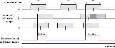
Support computation for three items a, b, c. Each event has an influence map (represented as a rectangle). If two influence maps overlap, their maximum (union) is computed. (In the diagram, item b has two events, the influence regions of which overlap.) The support results from the integral over the minima of the influence maps (intersections).
The divide-and-conquer scheme can be characterized roughly as follows: for a chosen item i, the problem to find all frequent patterns is split into two sub-problems: (1) find all frequent patterns containing item i and (2) find all frequent patterns not containing i. Each sub-problem is then further divided based on another item j: find all frequent patterns containing (1.1) both i and j, (1.2) i but not j, (2.1) j but not i, (2.2) neither i nor j etc.
In order to reduce the output we restrict it to closed frequent patterns. A pattern is called closed if no super-pattern has the same support. Closed patterns have the advantage that they preserve knowledge of what patterns are frequent and allow us to compute the support of any non-closed frequent pattern easily (see, for example, 2). However, it should be noted that the restriction to closed patterns is less effective with graded synchrony than with binary synchrony, because adding an item can now reduce the support not only by losing instances, but also by worsening the precision of synchrony. As a consequence, most patterns are closed under graded synchrony.
3. Jaccard Item Mining
As stated in the introduction, the objective of this paper is to develop a methodology that not only considers the number of synchronous events and the precision of their synchrony (like the synchrony operator does that we reviewed in the preceding section). Rather we want to be able to take into account whether the items have a low or high occurrence rate. The reason is that the same number of synchronous occurrences of a set of items can be significant for items with generally low occurrence rates, but explainable as a chance event for items with generally high occurrence rates, simply because high occurrence rates create more and larger chance coincidences.
For the transactional setting, such a behavior can be achieved by an approach that relies on item cover similarity measures instead of standard support 24. This approach is also referred to as Jaccard item set mining, because the most natural basis for an item cover similarity measure is the Jaccard index 13, which is a statistic for comparing sets. In the general case, for two arbitrary sets A and B, the Jaccard index is defined as
In frequent item set mining, the sets we consider are the so-called covers of items and item sets. Given transaction database T = (τ1,. . ., τm) over an item base B (that is, ∀k ∈ {1,. . ., m} : τk ⊆ B), the cover KS(I) of an item set I is defined as KS(I) = {k ∈ {1,. . .,m} | I ⊆ τk}, that is, as the set of indices of transactions that contain I. Analogously, the carrier LT (I) of an item set I is defined as LT (I) = {k ∈ {1,. . .,m} | I ∩ τk ≠ 0}24, that is, as the set of indices of transactions that contain at least one item in I. Note that the support is sT (I) = |KT (I)| and the extent is rT (I) = |LT (I)|24.
The core idea of using the Jaccard index for item set mining lies in the insight that the covers of (positively) associated items are likely to have a high Jaccard index, while a low Jaccard index indicates independent or even negatively associated items. However, since we are considering item sets of arbitrary size, we need a generalization of the Jaccard index to more than two sets. Following 24, we define such a generalized Jaccard index as
Using influence maps, this definition can easily be transferred to the continuous setting we consider here. We define a continuous item cover as
Since the support s𝒮,w(I) is obviously anti-monotone and the extent r𝒮,w(I) obviously monotone (that is, ∀I ⊆ J ⊆ B: r𝒮,w(I) ≤ s𝒮,w(J); or in words: if an item is added to an item set, its extent cannot decrease), we infer that the Jaccard index is anti-monotone, that is,
Given a user-specified minimum Jaccard value Jmin, an item set is called Jaccard-frequent iff J𝒮,w(I) ≥ Jmin. Since the Jaccard measure has essentially the same properties as the influence map overlap support defined in the preceding section, we can apply the same frequent item set mining scheme.
As an example consider Figure 1 again, namely for the computation of the support (numerator of the Jaccard index) of the set {a, b, c}, and Figure 2 for the computation of its extent (denominator of the Jaccard index), which results from the union of all influence maps of all involved items. Therefore, for the example shown in these two figures, we obtain
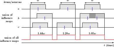
Additional computations for the Jaccard index for three items a, b, c (cf. Figure 1). The extent results from the integral over the maxima of the influence maps (union). The resulting Jaccard index is
Note that apart from the Jaccard index there are many other similarity measures for sets that can be generalized beyond pairwise comparisons and which also yield anti-monotone item cover similarity measures 24. All of these measures are defined in terms of the five quantities listed in Table 1 (which refers to the transactional setting). We already saw how the quantities sT (I) and rT (I) can be transferred and thus also know how to compute an analog of qT (I). The only problem is the quantity nT , the total number of transactions. In order to transfer this, we have to restrict our considerations in the continuous case to a finite recording period [ts, te], to which all integrals are then constrained. With such a constraint, we can define
| quantity | behavior |
|---|---|
| nT | constant |
|
|
anti-monotone |
|
|
monotone |
| qT (I) = rT(I) − sT(I) | monotone |
| oT (I) = nT − rT(I) | anti-monotone |
Quantities in terms of which the considered similarity measures are specified.
This allows, in principle, to transfer all item cover similarity measures considered in 24 to the continuous setting. However, we confine ourselves here to those measures that are derived from the inner product (listed in Table 2), and neglect those that are derived from the Hamming distance. The reason is that in our motivating application domain (spike train analysis) only the joint presence of spikes (as captured by s𝒮,w (I)) is considered as an indicator of joint processing of information, but not the joint absence of spikes (as captured by o𝒮,w(I), which occurs in addition in the numerator of similarity measures derived from the Hamming distance). Note also that the first measure in Table 2 (Russel&Rao) is merely a normalized form of the influence map overlap support defined in the preceding section.
| Russel & Rao23 | |
| Kulczynski17 | |
| Jaccard13 Tanimoto28 |
|
| Dice7 Sørensen27 Czekanowski5 |
|
| Sokal & Sneath25,26 | |
Considered similarity measures for sets/binary vectors.
Finally, note that the influence maps could, in principle, be generalized beyond rectangular functions as we use them in this paper. Even though it might not be so easy to justify the use of triangular or trapezoidal shapes in a meaningful way, there may be applications were such a generalization could be useful. In this case, the minimum of the influence maps (for their intersection) could be replaced by any t-norm and their maximum (for their union) by any t-conorm (see 15 for a comprehensive overview of t-norms and t-conorms). Alternatively, overlap functions as suggested in 4 could be used, generalized in a similar way to more than two arguments.
4. Pattern Spectrum Filtering and Pattern Set Reduction
The large number of patterns in the output of synchronous pattern mining is a general problem and thus further reduction is necessary. This is achieved by identifying statistically significant patterns. Previous work showed that statistical tests on individual patterns are not suitable 21,29. The main problems are the lack of proper test statistics as well as multiple testing, that is, the huge number of patterns makes it very difficult to control the family-wise error rate, even with control methods like Bonferroni correction, the Benjamini-Hochberg procedure, the false discovery rate etc. 8.
To overcome this problem, we rely here on the approach suggested in 21 and refined in 29, namely Pattern Spectrum Filtering (PSF). This method is based on the following insight: even if it is highly unlikely that a specific group of z items co-occurs s times, it may still be likely that some group of z items co-occurs s times, even if items occur independently. From this insight it is inferred that patterns should rather be judged based on their signature 〈z, s〉, where z = |I| is the size of a pattern I and s its support. A pattern is not significant if a counterpart, which has the same or larger pattern size z and the same or higher support s, can be explained as a chance event under the null hypothesis of independent events.
In order to determine the likelihood of pattern signatures 〈z, s〉 under the null hypothesis of independent items, a data randomization or surrogate data approach is employed. The general idea is to represent the null hypothesis implicitly by (surrogate) data sets that are generated from the original data in such a way that their probability is (approximately) equal to their probability under the null hypothesis. Such an approach has the advantage that it needs no explicit data model for the null hypothesis, which in many cases (including the one we are dealing with here) may be difficult to specify. Instead, the original data is modified in random ways to obtain data that are at least analogous to those that could be sampled under conditions in which the null hypothesis holds. An overview of several surrogate data methods in the context of neural spike train analysis can be found in 18.
In a nutshell, the idea of pattern spectrum filtering consists in collecting, for each pattern size z, the largest support value that was observed in the surrogate data sets for patterns of this size. Of the patterns obtained from the actual data set to analyze only those are kept that have a support larger than this maximum for their size. Note that since we are working in a continuous time domain, the support values are (non-negative) real numbers.
Unfortunately, even after pattern spectrum filtering, many spurious patterns may remain. Such patterns are caused by an actual pattern interacting with background chance events, which gives rise to sub-set, superset and overlap patterns. Supersets result from items outside of an actual pattern occurring by chance together with some of the instances of the actual pattern. Subsets result from some of the items in the actual pattern occurring together, in addition to the instances of the actual pattern, as a chance event. Finally, overlap patterns result from items outside of an actual pattern co-occurring with some instances of the injected pattern and at least one chance event of a subset of the actual pattern.
In order to remove such spurious induced patterns, we draw on pattern set reduction (PSR), as it was proposed in 29 for time-binned data, and transfer it to our setting. The basic idea is to define a preference relation between patterns X and Y with Y ⊂ X ⊆ B. Only patterns to which no other pattern is preferred are kept. All other patterns are discarded.
The preference relations considered in 29 are based on three core principles: (1) explaining excess coincidences (subsets), (2) explaining excess items (supersets) and (3) assessing the pattern probability based on the number of covered events. More formally, let zX = |X| and zY = |Y | be the sizes of the patterns X and Y, respectively, and let sX = s𝒮,w(X) and sY = s𝒮,w(Y ) be their support values. Since we have Y ⊂ X it follows zX > zY and sY > sX, because support is anti-monotone and we consider only closed patterns. With (1), X is preferred to Y if the excess coincidences sY − sX that Y exhibits over X can be explained as a chance event. With (2), Y is preferred to X if the presence of zX − zY excess items that X contains over Y can be explained as a chance event. With (3), the pattern is preferred for which z · s (or, alternatively, (z − 1) · s) is larger. In the case of time-binned data or binary synchrony, z · s is the number of individual events supporting a pattern. In the alternative version, the events of a reference item, to which the events of the other items are synchronous (as it makes no sense to speak of synchronous events if there is only one item), are disregarded.
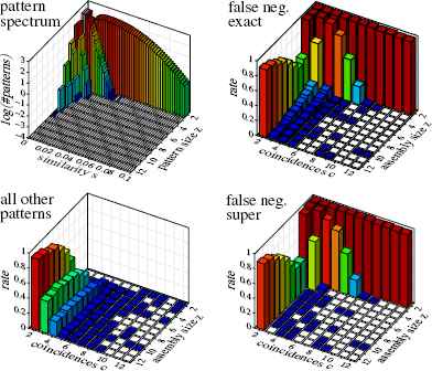
Transferring (1) and (2) to the case of graded synchrony turns out to be difficult, because the decision whether excess coincidences or excess items can be explained as chance events is made based on the pattern spectrum, using heuristic signature modifications that are tricky to transfer to a non-integer support. In addition, they are based on pairwise pattern comparisons, while the third approach relies on a potential function (in the sense of physics), thus simplifying the reduction process (see Section 5). As a consequence, we focus here on the third method, even though its intuitive justification as a number of events is also lost. However, we argue that the product of size (or size minus 1) and support can also be justified as derived from the shape of the decision border between significant and non-significant patterns as it is induced by the pattern spectrum. This border generally has a hyperbolic shape and is derived, in the binary case, from curves of pattern signatures having equal probability under certain simplifying assumptions (see 29). For this paper a visual inspection of a pattern spectrum as it is shown at the top left of Figures 3 and 5 may suffice as an intuition: The border between the white rectangles (pattern signatures that do no occur) and the rectangles with colored bars (pattern signatures occur with frequencies that are indicated by the bar heights and the bar colors) has a roughly hyperbolic shape.
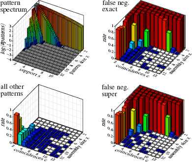
Experimental results with influence map overlap support: pattern spectrum and detection performance. Trial runs in which patterns other than the actual (injected) pattern are returned are few and concern mainly patterns with few coincidences, where a superset may be detected. Details about these additional patterns (divided into supersets, subsets, overlap and unrelated patterns) are depicted in Figure 4.
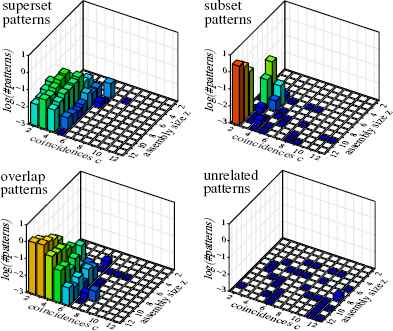
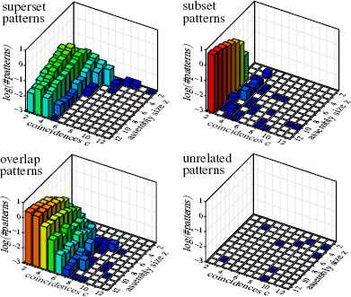
Experimental results with influence map overlap support: average numbers of patterns other than the actual (injected) pattern per data set. These patterns may be produced instead of or in addition to the actual (injected) pattern. Especially overlap patterns are usually returned in addition, as can be seen by comparing the diagram with the false negative diagrams in Figure 3.
Results with Jaccard similarity: pattern spectrum and detection performance. Note the lower number of false negatives compared to Figure 3. Trial runs in which patterns other than the actual (injected) pattern are returned are still few and concern mainly patterns with few coincidences, where a superset may be detected. Details about these additional patterns (divided into supersets, subsets, overlap and unrelated patterns) are depicted in Figure 6.
However, the graded synchrony we employ in this paper forces us to adapt this function. The reason is that with graded synchrony increasing the pattern size generally reduces the support, and not necessarily because instances get lost, but because the precision of synchrony is reduced by added items. This needs to be taken into account in the evaluation function. Since the loss of synchrony depends on the number of items, we heuristically chose (z − 1) (s + kz), where k is a (user-specified) parameter that is meant to capture the loss of synchrony relative to the pattern size.
5. Implementation Aspects
Having presented the theory of our method, we briefly consider some implementation aspects. The search for frequent synchronous patterns follows essentially the schemes of the Eclat algorithm for frequent item set mining 31 and of the JIM algorithm for mining Jaccard item sets 24. These algorithms work with a vertical representation of the transaction database, that is, they list for each item (or item set) the identifiers of the transactions in which the item (or item set) occurs. This approach is translated to a continuous (time) domain by collecting for each item (or item set) the intervals (of points in time) that are covered by an influence map (of a single item or of all items in the considered set). Like in Eclat or JIM these interval lists are processed by intersecting them to obtain the interval list (and thus the support) for the union of the item sets they refer to.
While this transfer is straightforward, it takes slightly more consideration how to obtain the extent r𝒮,w(I) of an item set I. There are two basic options: one can represent the carrier L𝒮,w(I), which is the union of the interval lists representing the influence maps of the items in I, or one can represent the complement of L𝒮,w (I), which is the intersection of the complements of the interval lists representing the influence maps of the items in I, since the total length of the intervals in the complement of L𝒮,w (I) is o𝒮,w (I), which is obviously related to r𝒮,w(I) by r𝒮,w(I) = n𝒮,w(I) − o𝒮,w(I).
In the transactional setting that is considered in JIM, the same two options exist in principle, but under normal conditions it is relatively clear that the second option is preferable, because the intersection becomes smaller with a growing number of items (fewer transactions do not contain any of the items) while the union grows with the number of items (more transactions contain at least one of the items). Since the length of the transaction identifier lists is decisive for the speed of the processing, intersection is preferable, because it leads, at least for larger item sets, to shorter lists.
In a continuous domain, however, the situation is different, because we work with interval lists instead of transaction identifier lists. This leads immediately to the observation that in terms of the lengths of these lists, there is no fundamental advantage for either choice, since the interval list representing the carrier L𝒮,w (I) and the list representing its complement can differ in length by at most one. The reason is that any interval end in the carrier is necessarily an interval start in its complement and vice versa. A difference can only result from the interval start that is the start of the recording period and the interval end that is the end of the recording period as these have no counterpart in the other list. If these two points occur in the same interval list (either both in the carrier L𝒮,w (I) or both in its complement), the corresponding list contains one interval more than the other, otherwise the number of intervals in both lists is exactly the same.
Since the length of the lists cannot be used to choose between the options, we wrote a test program to measure whether it is faster to merge two interval lists (forming the union of the contained intervals) or to intersect their complements. Since the program code for these two operations is considerably different, a speed advantage may result for one of the options. This is indeed what we found: over a wide range of parameters controlling, for instance, the size of the intervals versus the size of the gaps we found that computing the union is between 10% to 35% faster than computing the intersection of their complements, with the speedup most of the time falling into the range 20–25%. Due to this clear advantage, we chose to implement interval list merging to compute the extent r𝒮,w (I), in contrast to JIM, which intersects the complements of transaction identifier lists.
Note that, by analogy, this result could trigger us to compute the support s𝒮,w (I) not by intersecting the interval lists representing the influence maps of the items, but by merging their complements, exploiting that the total length of the intervals in this union represents o𝒮,w (I) + q𝒮,w (I) and thus allows to compute s𝒮,w (I) as s𝒮,w (I) = n𝒮,w (I) − o𝒮,w (I) − q𝒮,w(I). However, we maintained the intersection, because the complement can only be used if the recording period is fixed, but with intersection, influence map overlap support alone can be computed without this knowledge (ignoring that, in principle, one may not want to consider the part of an influence map that extends before the start or after the end of the recording period).
Another implementation aspect concerns pattern set reduction, which was generally introduced in 29 based on a preference relation between patterns, one of which is a subset of the other. If the preference relation can only be evaluated by looking at every pair of patterns explicitly (as it is the case for some of the methods proposed in 29), the complexity of this step is quadratic in the number of patterns. Unfortunately, in our setting we have to deal with many more patterns (sometimes thousands to tens of thousands after pattern spectrum filtering), mainly because there are fewer non-closed patterns: (1) influence map overlap support already tends to change with the addition of an item, because it captures not only the number of coincidences (which may stay the same), but also the precision of synchrony (which may be reduced by the additional item) and (2) even if the support of an item set is not affected by adding an item, the extent of the item set almost certainly changes, thus affecting basically any item cover similarity measure.
To cope with this problem, we employed in 9 only preference relations that assign a numeric value to each pattern (potential function) and establish a preference by simply comparing these values. This allows for a faster pattern set reduction scheme: the patterns are sorted descendingly w.r.t. the value assigned to them and all patterns are marked as selectable. Then the following candidate selection is repeated until no selectable patterns remain: the selectable pattern with the highest evaluation is marked as a candidate and all subsets of this pattern that are further down in the list are marked as excluded. This leaves a (usually considerably) reduced list of candidate patterns, which is further reduced as follows: for each candidate pattern it is checked whether there exists (among all patterns, including the ones marked as excluded) a subset with a better evaluation. If such a subset exists, the candidate pattern is marked as excluded. Finally only the patterns not marked as excluded are returned. Although this procedure still has quadratic time complexity in the worst case, it is usually much faster in practice.
6. Experiments
In order to test our algorithm, we generated artificial data sets, so that we know what can (and should) be found in these data sets. Using real-world data sets at the stage of method development (and this is what we do here: we develop a method to effectively and efficiently detect statistically significant synchronous activity in sequence data) is not possible, because for a real-world data set—especially from the area of neural spike train analysis, our motivating application area—no one can tell (yet) what a correct result would be. However, the parameters we used for generating data sets are inspired by the properties of actual parallel neural spike trains and the current technological possibilities for recording them: we consider 100 items (or neurons), which is in line with the sizes of current multi-electrode arrays, a recording length of 3s (in neurobiological practice recording times range from a few seconds to about half an hour), and an average item rate of 20Hz, which is a typical average physiological firing rate of biological neurons.
Since our objective is to improve the sensitivity of detecting synchronous spiking in groups of neurons with a (comparatively) low firing rate in the presence of neurons with a (much) higher firing rate, we split the 100 items into 4 groups with 25 items each and item occurrence rates of 8, 16, 24, and 32Hz, respectively (thus obtaining an over-all average rate of 20Hz). All item occurrences are generated as independent stationary Poisson processes. Starting from this basic setup we generate 1000 data sets for each pattern signature 〈z, c〉 ∈ {2, . . ., 12}2, injecting a pattern with that signature into the group of 25 items with 8Hz occurrence rate. This is done by sampling c points in time uniformly from the recording period of 3s, which are then jittered for each of the z items individually by adding random offsets that are sampled from the interval [−1ms, +1ms]. The remaining (background) item occurrences are generated as independent stationary Poisson processes with rates (8 −c/3)Hz (where the 3 refers to the recording period length of 3s), thus obtaining a combined item occurrence rate of 8Hz.
Note, however, that this does not mean that our method focuses solely on detecting synchronous activity among the items in this group (for which we could just as well restrict the analysis to this sub-group, with possibly better results). Our method rather places no restrictions on the combinations of items, so that any mixture of items with high or low occurrence rates could constitute a pattern, which our method would be able to detect. We merely chose to inject synchronous activity into the group with lowest rate, because this demonstrates the advantages of our method most distinctly.
For each data set with an injected pattern we mined (closed) frequent synchronous patterns with the extended version of CoCoNAD we developed, using influence map overlap support or (also) item cover similarity to guide the search. We employed an influence map width of 3ms and a minimum support threshold of 1 (in accordance with the choices in 9), while no minimum item cover similarity threshold was employed. That is, we effectively mined the same set of patterns in both cases, but en-dowed them with the additional information of the item cover similarity in the latter.
For pattern spectrum filtering we generated 10,000 independent data sets with the same parameters stated above, but without any injected synchronous patterns. These data sets were mined for (closed) frequent synchronous patterns with the extended version of CoCoNAD we developed, in essentially the same way as we mined the data sets with injected patterns (influence map width 3ms, minimum support threshold 1, cf. 9). For each pattern size we recorded the largest item cover similarity (or largest influence map overlap support, respectively) that occurs for patterns of this size. These values constitute the significance decision border: any pattern in the data to analyze that achieves a higher item cover similarity (or influence map overlap support, respectively) than the maximum observed for the same pattern size in any of these data sets will be labeled significant.
Note that, in a strict sense, this procedure is a shortcut, because in principle we should generate new surrogate data sets for each of the data sets with an injected pattern. However, since with the described setup we have to analyze 121,000 data sets (11 sizes × 11 numbers of coincidences × 1000 data sets), generating several thousand separate surrogate data sets for each of them is impossible. In order to obtain a feasible procedure, we use the single pattern spectrum derived from the 10,000 independent data sets for all detection runs. This is admissible, because all of these data sets share the same basic properties (same parameters) and therefore the differences between using a pattern spectrum derived from such independent data sets or one derived from specific surrogate data sets are negligible.
The remaining patterns are reduced with pattern set reduction, using (z − 1) · (c + 0.15z) as the evaluation measure (in accordance with 9) for both setups. That is, even if item cover similarity was used for pattern spectrum filtering, the remaining patterns were reduced based on influence map overlap support. The reason for this choice is that experiments in which we tried to base pattern set reduction on item cover similarity as well always produced somewhat worse results. With the reduced pattern set it is then checked whether the injected pattern was found and what other patterns were returned instead of or in addition to the injected pattern.
The results are depicted in Figures 3 to 6, of which the first two refer to influence map overlap support and the latter two to item cover similarity. Since all of the item cover similarity measures we tried (Jaccard/Tanimoto, Kulczynski, Dice/Sørensen/Czekanowski, Sokal&Sneath) produced almost the same results, we only show the results for the Jaccard measure. However, the complete set of results can found on the web page stated in section 8.
Results with Jaccard similarity: average numbers of patterns other than the actual (injected) pattern per data set. These patterns may be produced instead of or in addition to the actual (injected) pattern. Especially overlap patterns are usually returned in addition, as can be seen by comparing the diagram with the false negative diagrams in Figure 5. More patterns compared to Figure 4 occur mainly where no detection was possible with influence map overlap support.
As can be seen in Figures 3 and 4, the detection quality is already fairly good with influence map overlap support, provided the injected pattern is sufficiently large or exhibits sufficiently many synchronous events. However, compared to the results in 9, in which all 100 neurons had the same firing rate of 20Hz, a larger pattern size or more coincidences are needed for a reliable detection. The reason for this is, of course, that the items with a larger firing rate increase the decision border by producing more and larger chance coincidences, which make the pattern detection more difficult.
In contrast, the results based on item cover similarity show a much larger sensitivity, especially for patterns with 3 to 5 items, which are detected with considerably fewer coincidences, as can be seen from a comparison of Figures 5 and 3. Alternatively, we may say that patterns can be detected with about two items less than with influence map overlap support.
However, at first sight, a comparison of Figures 6 and 4 seems to indicate that this improvement comes at the price of more patterns that are not the injected one (like subsets, supersets and overlap patterns). However, a closer look reveals that these additional patterns occur mainly for pattern signatures for which an influence map overlap support does not produce any output at all. Clearly, it is preferable to detect actually present patterns at the price of a few subset or overlap patterns in some runs. Note also that the vertical axis has a logarithmic scale and thus that in most cases in 90% of all runs no subset pattern is produced. Merely overlap patterns become slightly more frequent, though mainly for very low numbers of coincidences.
In order to give a rough idea of the execution times needed by our methodology, we report some time measurements from our experiments as we described them above, Table 3. *However, we caution a reader not to over-interpret these numbers. Actual execution times on specific data sets differ widely, depending on the parameters of the data (like the number of neurons, their firing rates, the chosen window width, the patterns that are contained etc.). In order to get a better idea of execution times on data a reader wants to apply our method to, we refer to the software we made publicly available (see below), with which concrete experiments can easily be carried out. The times show that at least for the parameters we chose the execution is very fast and usually consumes only a fraction of a second per detection run. If the patterns become larger, both the computation of the similarity measure as well as the pattern set reduction (mainly the latter) lead to increases of the computation time. However, at least in this context, the execution times stay within very reasonable limits and thus it should not be too problematic to enlarge the window width if required.
| without injected patterns | ||
|---|---|---|
| width w | cov.sim. | execution time |
| 3.0ms | none | 36.08ms |
| 3.0ms | Jaccard | 51.48ms |
| 4.5ms | none | 92.29ms |
| 4.5ms | Jaccard | 139.14ms |
| with one injected pattern | |||||
|---|---|---|---|---|---|
| width w | cov.sim. | jitter | pat.size z | #coins. c | execution time |
| 3.0ms | none | 2.0ms | 8 | 8 | 45.04ms |
| 3.0ms | Jaccard | 2.0ms | 8 | 8 | 64.92ms |
| 3.0ms | none | 2.0ms | 12 | 12 | 114.15ms |
| 3.0ms | Jaccard | 2.0ms | 12 | 12 | 594.63ms |
| 4.5ms | none | 3.0ms | 8 | 8 | 111.86ms |
| 4.5ms | Jaccard | 3.0ms | 8 | 8 | 171.90ms |
| 4.5ms | none | 3.0ms | 12 | 12 | 252.33ms |
| 4.5ms | Jaccard | 3.0ms | 12 | 12 | 1707.98ms |
Execution times of individual detection runs on data sets with the parameters stated in the text. All times were computed as averages over 1000 runs. The top table records execution times of runs for establishing a pattern spectrum (that is, on data without injected patterns) while the bottom table shows execution times for data with injected patterns with two different pattern signatures. The pattern set reduction was carried out with the methods that we found to be best (see text).
7. Conclusions
We presented an extension of the CoCoNAD algorithm and its accompanying methodology to single out significant and relevant synchronous patterns with the help of pattern spectrum filtering (PSF) and pattern set reduction (PSR) that improves the detection sensitivity by taking the individual item rates into account. This is achieved by basing pattern spectrum filtering upon item cover similarity measures (like the Jaccard index) transferred to a continuous (time) domain. The core idea is that in this way the ratio of coincident occurrences to the total number of occurrences of some items (rather than merely the number of coincident occurrences and their precision of synchrony) determines whether a synchronous event is significant or not. Detection sensitivity is thus improved, because the same number of occurrences can be a chance event among items having high occurrence rates, but a (statistically) significant event among items having low firing rates. Pattern set reduction still employs influence map overlap support, though, because for comparing filtered patterns the number of synchronous events and the precision of synchrony is better suited than an item cover similarity measure. This combined methodology leads to a considerable improvement if patterns are potentially disguised by (many) items with a high occurrence rate, as we demonstrated with extensive experiments on artificial data sets.
8. Software and Result Diagrams
The described variant of the CoCoNAD algorithm is available as a command line program ccn-ovl as part of the basic CoCoNAD package
The Python scripts with which we conducted our experiments as well as the full set of result diagrams we produced can be found at
With the efficient implementation of the command line program as well as the Python extension library, a single analysis run (one data set) in our experiments takes only a fraction of a second. The most costly part is the generation of the pattern spectrum, since it involves analyzing 10,000 data sets, but even this takes only a few minutes. Running the whole set of experiments, however, can take several hours, due to the huge number of data sets (> 100, 000) that need to be generated and analyzed in several ways.
Acknowledgements
The presented research was performed under no affiliation and only as a personal purpose of the authors.
Footnotes
All experiments were run on an Intel Core 2 Quad Q9650@3GHz system with 8GB of main memory under Ubuntu Linux 16.04; the Python extension library—written in C—was compiled with gcc 5.3.1, the scripts were executed with Python 2.7.11.
References
Cite this article
TY  - JOUR
AU  - Salatiel Ezennaya-Gomez
AU  - Christian Borgelt
PY  - 2018
DA  - 2018/01/22
TI  - Mining Frequent Synchronous Patterns based on Item Cover Similarity
JO  - International Journal of Computational Intelligence Systems
SP  - 525
EP  - 539
VL  - 11
IS  - 1
SN  - 1875-6883
UR  - https://doi.org/10.2991/ijcis.11.1.39
DO  - 10.2991/ijcis.11.1.39
ID  - Ezennaya-Gomez2018
ER  -