
A dynamic multi-attribute group emergency decision making method considering experts’ hesitation
- DOI
- 10.2991/ijcis.11.1.13How to use a DOI?
- Keywords
- Multi-attribute group decision making; Emergency situation; Dynamic evolution; Experts’hesitation
- Abstract
Multi-attribute group emergency decision making (MAGEDM) has become a valuable research topic in the last few years due to its effectiveness and reliability in dealing with real-world emergency events (EEs). Dynamic evolution and uncertain information are remarkable features of EEs. The former means that information related to EEs is usually changing with time and the development of EEs. To make an effective and appropriate decision, such an important feature should be addressed during the emergency decision process; however, it has not yet been discussed in current MAGEDM problems. Uncertain information is a distinct feature of EEs, particularly in their early stage; hence, experts involved in a MAGEDM problem might hesitate when they provide their assessments on different alternatives concerning different criteria. Their hesitancy is a practical and inevitable issue, which plays an important role in dealing with EEs successfully, and should be also considered in real world MAGEDM problems. Nevertheless, it has been neglected in existing MAGEDM approaches. To manage such limitations, this study intends to propose a novel MAGEDM method that deals with not only the dynamic evolution of MAGEDM problems, but also takes into account uncertain information, including experts’ hesitation. A case study is provided and comparisons with current approaches and related discussions are presented to illustrate the feasibility and validity of the proposed method.
- Copyright
- © 2018, the Authors. Published by Atlantis Press.
- Open Access
- This is an open access article under the CC BY-NC license (http://creativecommons.org/licences/by-nc/4.0/).
1. Introduction
With the increasing occurrence of various emergency events (EEs)—such as production accidents, natural disasters, and terrorist attacks—emergency decision making (EDM) has drawn wide attention across the world in the past few years, and especially due to its prominent part in reducing the property loss and casualties in different EEs. Hence, it has become a pressing and important research topic10,18,29,31.
When an EE occurs, the information related to it changes across time, leading to dynamic evolution. Furthermore, its information is usually uncertain, especially in the early stages. Therefore, EE information plays an important role in the EDM process; it is necessary to take into account both its dynamic evolution and its uncertainty10,29 to deal with it satisfactorily.
For executing effective emergency responses using updated information to control the situation and mitigate losses caused by EEs, the dynamic evolution13,29 and uncertain information14,31 features have been already discussed in current EDM approaches. Nevertheless, these studies13,29 examines dynamic evolution considering only time changes; the information regarding the alternatives and criteria13,29 remain unchanged, even though the EE information changes along with the time. Discrete and dynamic decisions with the latest information might make the EDM more effective and appropriate. On the other hand, current EDM approaches deal with the uncertain information using interval values31 for quantitative contexts, and linguistic term sets 14 for qualitative contexts. However, due to lack of information and time pressure in EDM, decision makers might hesitate when they have to assess the alternatives and criteria. Thus, hesitant information should be considered in these types of problems 27.
Usually, in classical EDM approaches10,13,14,18,29,31, only one emergency decision maker (DM) is in charge of the EE. However, it is highly challenging for an individual DM 19 to deal with these complicated emergency situations in real world problems. Consequently, multi-attribute group emergency decision making (MAGEDM) might be a powerful and effective way to cope with complex and damaging EEs. A general scheme of a MAGEDM problem is shown in Fig. 1.
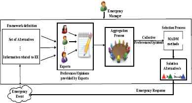
General scheme of a MAGEDM problem
MAGEDM is a vital decision activity for dealing with real world EEs11,16,30, wherein experts play the role of think tanks to provide their opinions or assessments of different alternatives regarding different criteria; experts’ individual wisdoms are aggregated into a group to help the DM make a final decision.
As far as we know, until now, no proposal in current MAGEDM approaches 35,36,37,38 considers the dynamic evolution of EEs dealing with both the updated information about alternatives and criteria along with the time and the experts’ changes (quit or invited to join in the decision process), in addition to the modelling of experts’ hesitancy due to uncertain information. Therefore, it is practically significant to address these issues in order to make satisfactory and reasonable decisions in real world MAGEDM problems.
This study aims to develop a new dynamic MAGEDM method that deals with the dynamic evolution of EEs considering both the time changeableness and updated information (alternatives, criteria, and experts). At the same time, it deals with uncertain information by using interval values, linguistic term sets, and linguistic expressions based on hesitant fuzzy linguistic term sets (HFLTS)27, which are able to model experts’ hesitancy.
In dynamic MAGEDM problems, the alternatives are ranked according to the dynamic rating of each alternative at different decision moments. Dynamic rating of each alternative is usually determined by the static rating of the alternative at the current decision moment and its dynamic rating in previous one 4. Therefore, the ranking obtained by using the dynamic ratings could be different from the static ratings. Static ratings are usually obtained by using different multi-attribute decision making methods (MADM)3,42. In order to retain uncertain information as much as possible and generate more reasonable decision results, fuzzy TOPSIS method based on alpha-level sets is regarded as the static MADM method in the proposal to obtain the static rating of alternatives at each decision moment because of its capacity and advantages of using uncertain information across the decision process.
The rest of this paper is organized as follows: Section 2 briefly introduces different concepts that will be used in the proposed method. Section 3 presents a novel dynamic MAGEDM method considering experts’ hesitancy. In section 4, a case study is introduced, and comparisons with current approaches and related discussions are presented. The conclusions and prospective research areas are offered in section 5.
2. Preliminaries
This section briefly revises basic concepts regarding imprecise and hesitant information and dynamic decision making to understand the proposed dynamic MAGEDM method easily. It also introduces the fuzzy TOPSIS method based on alpha-level sets, which will be utilized as the static MADM in the computing static rating process in our proposal to obtain the static rating of alternatives at each decision moment.
2.1. Dealing with imprecise and hesitant information
Uncertain information is one of the remarkable features of EEs. It is very important to deal with such type of information to cope with EEs successfully. Therefore, information domains utilized by experts to provide their opinions/assessments in quantitative and qualitative contexts are revised.
(1) Information domain for quantitative contexts
In real world problems, it is difficult for experts to provide their assessments using numerical values, when the EE information is uncertain, such as people affected, property losses, or costs of alternatives. However, in such situations, interval values15,22,31 are suitable for experts to provide their assessments due to their useful and simple technique for representing uncertainty. Thus, interval values are utilized as the information domain for quantitative contexts in our proposal.
Definition 1. 23
Let [ηL, ηU] be a domain of the interval value; an interval value I belongs to [ηL, ηU]:
(2) Information domain for qualitative contexts
A fairly common approach to model qualitative information is the fuzzy linguistic approach39 based on the fuzzy set theory. Different linguistic models have been discussed in different approaches20,21,26. In our proposal, linguistic term sets are utilized to model the uncertain information in qualitative contexts (see Fig. 2).
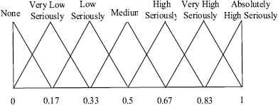
Linguistic term set
Definition 2. 27
Let S = {s0, s1, …, sg} be a linguistic term set; a linguistic term, si, belongs to S:
Usually the information of MAGEDM problems is uncertain; experts involved in such problems are bounded by cognition 2 and under pressure because of the urgent time constraints in an emergency response. Moreover, their decision might provoke potentially serious results 16. Hence, in such situations, it is common for experts to hesitate when they provide their assessments. Therefore, it seems necessary to deal with experts’ hesitation in MAGEDM problems.
To model the hesitant information in qualitative contexts, the concept of HFLTS 27 was introduced, drawing increased attention recently 25,27.
Definition 3. 27
Let S = {s0,s1, …, sg} be a linguistic term set; a HFLTS, HS, on S is an ordered finite subset:
Example 1.
Let S={absolute weak, very weak, weak, medium, good, very good, excellent} be a linguistic term set and δ be a linguistic variable; then,
HFLTS is a powerful and useful tool to model experts’ hesitation; the use of context-free grammars 27 allows generation of complex linguistic expressions close to the natural language utilized by human beings in the real world 27,28, which can be modeled by HFLTS. This approach has been widely applied to deal with different decision problems 1,33,34.
Definition 4. 27
Let S = {s0, s1, ..., sg} be a linguistic term set and GH be a context-free grammar. The elements of GH = (VN , VT , I , P ) are defined as below:
={ 〈primary term〉, 〈composite term〉, 〈unary relation〉, 〈binary relation〉, 〈conjunction〉} = {lower than, greater than, at least, at most, between, and, s0,s1, …, sg} ∈ VN = {I:: = 〈primary term〉 | 〈composite term〉 〈composite term〉 :: = 〈unary relation〉 〈primary term〉 | 〈binary relation〉 〈primary term〉 〈conjunction〉 〈primary term〉 〈primary term〉 :: = s0 |s1|…|sg 〈unary relation〉 :: = lower than |greater than |at least |at most 〈binary relation〉 :: = between 〈conjunction〉 :: = and}
Sll denotes the expression domain generated by GH , which might be either complex linguistic expressions or single linguistic terms.
Example 2.
Considering the context-free grammar, GH, introduced in Definition 4 and the linguistic term set S from example 1, the following complex linguistic expressions might be obtained:
Sll1 = at least good
Sll2 = at most medium
Sll3 = between good and very good
Taking into account that experts can provide their assessments by utilizing quantitative and qualitative information in order to make computations with different types of information, it is necessary to unify them into a unique domain. The process of unifying different types of information is presented in section 3.3.
2.2. Dynamic decision making
Some existing dynamic MADM methods 3,4, which have the following remarkable features, are revised:
- (i)
The alternatives are changeable because they might be deemed non-available or removed; meanwhile new alternatives might be considered and added.
- (ii)
The criteria are not immobilized, since their values might change along with time, and also, the current criteria might be removed or new criteria might be taken into account.
- (iii)
According to these three features, dynamic MADM methods should be capable of managing interdependent decisions in a changing environment, wherein not only alternatives, but criteria might also change (non-available, removed or added new ones, etc.) and the final decisions at each decision moment must consider the feedback from previous ones. Due to the dynamic evolution of EEs, a reasonable and effective MAGEDM method should consider not only the three aforementioned features, but also the changes of experts because they might give up the decision process or new experts might be invited to join the decision process in real world situations.
To make the proposed MAGEDM method understandable, some necessary concepts are first given, and then the dynamic MADM method 3,4,42 is briefly revised.
Definition 5. 3 (Historical set)
The historical set of alternatives as decision moment, t ∈ T, is a subset of all alternatives that have ever been available up to and including that decision moment,
Remark 1. 3
In practical applications, the historical set is updated incrementally. Let H0 = ϕ, at each decision moment, t ∈ T. Then, the historical set can be defined as
Let T = {1, 2, …} set of discrete decision moments (possibly infinite), and Pt be the set of alternatives that are usable at each decision moment, t, t ∈ T. Suppose that a static MADM method is being utilized at each decision moment, t ∈ T, to compute ratings for each available alternative, p ∈ Pt, concerning the assessments of all criteria, Ct = {c1, c2, …, cm}. The ratings obtained by the static MADM method are called static ratings or non-dynamic ratings, denoted by Rt(p). The dynamic rating of alternatives is computed based on its static rating obtained in the previous stages to which it belonged.
The dynamic decision process deals with a feedback mechanism from previous ones. For any alternative, p, its dynamic rating function, Et(p),is defined as 3,4,42:
For each alternative, p, either belonging to the existing set of alternatives, Pt, or carried over from the previous one by means of the historical set, Ht−1, there are three different situations.
- (i)
if the alternative, p, belongs only to the current set of alternatives, Pt, but not to the historical set, Ht−1, that is, p ∈ Pt\Ht−1, its dynamic rating, Et(p), is equal to its static rating, Rt(p);
- (ii)
if the alternative, p, belongs not only to the current, but also the historical set of alternatives, that is, p ∈ Pt ∩Ht−1, its dynamic rating, Et(p), is calculated by aggregating its static rating, Rt(p), with its dynamic rating, Et−1(p), at the former decision moment; and
- (iii)
if the alternative, p, belongs to the historical set of alternatives only, that is, p ∈ Ht−1\Pt, its dynamic rating, Et(p), is equal to Et−1(p).
The dynamic decision process can be conducted for several decision moments. The moment wherein the process is stopped depends on the problem and the DM’s assessments.
2.3. Fuzzy TOPSIS method based on alpha-level sets
TOPSIS (Technique for Order Preference by Similarity to Ideal Solution) method was first proposed by Huwang and Yoon 12; it is a popular MADM method been widely applied to solve different decision problems 5,6,12,32. To cope with complex problems and uncertain information in the real world, the TOPSIS method has been extended to deal with fuzzy MADM problems 5,6,32.
The fuzzy TOPSIS method based on alpha-level sets 32 is a distinctive and powerful approach among other fuzzy TOPSIS versions 5,6,8,9 due to its prominent advantages of keeping uncertain information in a better way. This is the significant difference between the fuzzy TOPSIS method based on alpha-level sets and other versions. Due to such advantages, the fuzzy TOPSIS method based on alpha-level sets will be used as the static MADM method in order to calculate the static rating of each alternative at different decision moments in our proposal.
In fuzzy MADM problems, criteria/attribute values and the relative weights are usually characterized by fuzzy numbers 6,32. The most commonly used fuzzy numbers are trapezoidal fuzzy numbers, Ã = (a, b, c, d) or triangular fuzzy numbers, Ã = (a, b, d) with a degree of membership between 0 and 1. When b = c, the triangular fuzzy number is a special case of a trapezoidal fuzzy number.
According to Zadeh’s extension principle 41, a fuzzy number/set, Ã, can be also expressed by its intervals, that is,
Based on the short revision of fuzzy numbers aforementioned, the fuzzy TOPSIS method based on alpha-level sets 32 is briefly introduced.
Let
If
It can be seen that
Let
RCi is an interval value based on Eq. (15); its upper and lower bounds can be calculated by utilizing the following simplified pair of fractional programming models (see 32 for further details):
According to Eq. (6), the dynamic ratings of alternatives are related not only to their static ones, but also their performance in previous stages if it has one. In order to calculate the dynamic ratings of alternatives, it is firstly necessary to compute the static ratings of alternatives. The averaging level cuts 24 are used in this paper for sake of simplicity to obtain the static ratings of alternatives.
Let α1, …, αK be different alpha levels; the static rating,
3. Dynamic MAGEDM method considering experts’ hesitation
This section introduces a novel dynamic MAGEDM method that is able to: (a) consider the dynamic evolution feature of EEs in MAGEDM problems; and (b) deal with uncertain information using interval values in quantitative contexts, linguistic terms in qualitative contexts, and model experts’ hesitation by means of complex linguistic expressions based on HFLTS.
This proposal extends the general scheme of the MAGEDM process shown in Fig. 1 by adding two new phases to unify the information provided by experts (unification process), and then, compute the dynamic rating (computing dynamic rating). The aggregation process has been modified, and the selection process is replaced by a new phase adapted to dynamic MAGEDM problem (computing static rating). These phases are highlighted in Fig. 3 by using dash lines.
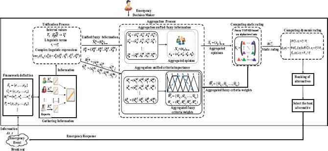
Dynamic MAGEDM method considering experts’ hesitation
The proposed dynamic MAGEDM method consists of six main phases:
- (a)
Framework definition. It defines the structure of the dynamic MAGEDM problem (notions for decision moments, experts, alternatives, etc.) and the expression domains for quantitative and qualitative contexts wherein assessments can be elicited by involved experts.
- (b)
Gathering information. Assessments of or opinions on different alternatives concerning different criteria and criteria importance are provided by experts at each decision moment.
- (c)
Unification process. The information provided by experts at each decision moment is unified into a fuzzy domain to carry out the computations.
- (d)
Aggregation process. In this process, the unified fuzzy information about the opinions, and criteria importance provided by experts are aggregated.
- (e)
Computing static rating. Fuzzy TOPSIS method based on alpha-level sets is utilized as the static MADM method to calculate the static rating of each alternative at each decision moment.
- (f)
Computing dynamic rating. Dynamic rating for each alternative at each decision moment takes into account not only its static rating in the current stage, but also its performance in previous ones.
These phases are further detailed in the following subsections.
3.1. Framework definition
The following notions and terminology will be used in the proposed dynamic MAGEDM method.
- •
T = {1, 2, 3, …}: the set of discrete decision moments (possible infinite), for each decision moment, t ∈ T.
- •
Pt = {p1, p2, …, pn}: the set of available alternatives at decision moment, t, where pi denotes the i-th alternative, i = 1, 2, …,n.
- •
Ct = {c1, c2, …, cm}: the set of criteria/attributes at decision moment, t, where cj denotes the j-th criterion/attribute, j = 1, 2, …, m.
- •
Et = {e1, e2, …, eH}: the set of experts at decision moment, t, where eh denotes the h-th expert, h = 1, 2, …, H . In dynamic MAGEDM problems, the experts might leave or be added during the decision process according to expert’s willingness or decision problems.
- •
- •
- •
Xt = (xij)n×m: denotes the aggregated information matrix regarding
- •
- •
- •
Remark 2.
The expression domains used by experts to express their assessments,
Remark 3.
The expression domains for the criteria importance are either single linguistic terms, si ∈ S , or complex linguistic expressions, Sll, because they are close to the natural language employed by people in real world.
3.2. Gathering information
The opinions/assessments,
3.3. Unification process
In this proposal, the expression domains used by experts can be interval values (I), linguistic terms (si), or complex linguistic expressions (Sll).
- •
Interval values. Assessments represented by interval values, I , belong to a special domain, [ηL, ηU], that is, I ∈ [ηL, ηU].
- •
Linguistic terms. Assessments represented by linguistic terms si, belong to a linguistic term set S = {s0, s1, …, sg}, that is, si ∈ S , where g + 1 is the granularity of S .
- •
Complex linguistic expressions. Assessments represented by Sll, generated by GH (see Definition 4).
As mentioned in section 2.1, to deal with quantitative and qualitative information, a unification process is needed to facilitate the computations.
In order to retain uncertain information, including experts’ hesitation, and obtain more reliable results, the assessments,
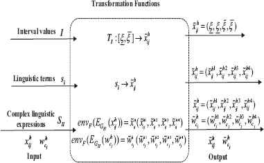
Transformation functions
The transformation functions are detailed below:
1) Interval values, I , are first normalized into [0,1], and then, transformed into trapezoidal fuzzy numbers by using a transformation function, TI . Let [ηL,ηU] be the domain of the interval values for quantitative contexts; let
The transformation function, TI , is defined as follows.
Definition 6.
Transformation function, TI , transforms an interval value into a trapezoidal fuzzy number:
2) Linguistic terms,
3) Complex linguistic expressions,
According to Eqs. (24)–(26), the gathered information,
3.4. Aggregation process
The aggregation process is the process wherein experts’ opinions are aggregated to obtain collective values for each alternative and criteria weights.
The unified information,
- 1)
Aggregation of unified fuzzy information.
The aggregated fuzzy information matrix at decision moment, t, Xt = (xij)n×m, where
where h = 1, 2, … , H ; i = 1, 2, …, n, j = 1, 2, … , m. - 2)
Aggregation of unified criteria importance.
The aggregated fuzzy criteria weights at decision moment, t,
where h = 1, 2, … , H , j = 1, 2, … , m.
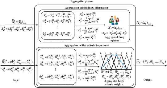
Aggregation process
The advantages of the aggregation equations above are not only to retain uncertain information as much as possible and take into account all involved experts’ opinions in the dynamic MAGEDM process, but also to ease computation.
3.5. Computing static rating
As noted earlier, the fuzzy TOPSIS method based on alpha-level sets is utilized as the static MADM method to obtain the static ratings of alternatives at each decision moment, t, in our proposal. Since the aggregated fuzzy information matrix, Xt = (xij)n×m and
Let
3.6. Computing dynamic rating
Since EE information changes along with time (alternatives, criteria, and experts), leading to dynamic evolution, it seems necessary to consider the dynamic rating of each alternative. This is a comprehensive factor that indicates the performance of the alternative not only in its current stage, but also in the previous one. In this proposal, the dynamic rating of alternatives based on Eq. (6) is as follows:
The operator selection and reinforcement depend on the characteristics of the problem.
Definition 7. 42
A probabilistic sum function, Φ, is defined as:
The ranking of the alternatives is obtained according to the dynamic ratings, Et(pi); the higher dynamic rating the better alternative.
4. Case study, comparison with other approaches and discussions
In order to illustrate the feasibility and validity of the proposed dynamic MAGEDM method, a case study adapted from a big explosion† that occurred in China is provided, followed by comparisons with other approaches and related discussions.
4.1. Case study
A big explosion took place at a container storage station at the Port of Tianjin, which contained hazardous and flammable chemicals, including sodium nitrate, calcium carbide, and ammonium nitrate, among others. The local government organized relevant departments (fire department, traffic management department, hygiene department, etc.) to collaborate in order to address the emergency situation. Short messages were sent to inform citizens within one kilometer to evacuate to safe areas. In this example, when the explosion occurred, the decision moment, t = 1.
4.1.1. Decision moment t=1
Step 1. Framework definition
Assume that three experts E1 = {e1, e2, e3} are invited to join in the MAGEDM process to help the DM to make a decision. Three available alternatives, P1 = {p1, p2, p3}, were put forward concerning three criteria, C1 = {c1, c2, c3}, which are given in Tables 1 and 2, respectively.
Alternatives Description p1 Inform and evacuate citizens, and meanwhile assign 10 fire squadrons, 300 fire fighters, and 40 fire engines to deal with the explosion. p2 Increase to 30 fire squadrons, 900 fire fighters, and 55 fire engines; at the same time, report the latest news to the citizens to avoid panic and riots. p3 Ask the professional emergency rescue military for emergency rescue with more than 300 soldiers carrying specific equipment join in the rescue. Table 1.Description of available alternatives at t = 1
Criteria Expression domain Description People affected (c1) I It means the alternative, pi, can protect the number of people from the effects caused by EE in domain [0,1000]. Environment affected (c2) S1, Sll It is evaluated by experts by using si ∈ S1 = {None (N), Very Low Seriously (VLS), Low Seriously (LS), Medium (M), High Seriously (HS), Very High Seriously (VHS), Absolutely High Seriously (AHS)} and Sll generated by GH on S1 (see Fig. 2). Property loss (c3) I It means that the alternative, pi, can protect the direct and indirect property losses caused by EE in domain [0,10] (in billion RMB). Table 2.Description of criteria at t = 1
Step 2. Gathering information
The criteria importance,
Criteria c1 c2 c3 VH1 H1 LI VH1 H1 LI VH1 bt MI and HI VLI Table 3.Criteria importance
The assessments,
Criteria c1 c2 c3 [50,80] VLS [0.3,0.5] [80,100] M [0.4,0.5] [45,55] M [0.25,0.35] [40,60] LS [0.2,0.3] [80,110] M [0.3,0.5] [30,40] HS [0.2,0.25] [50,60] LS [0.18,0.25] [70,120] M [0.45,0.6] [35,45] At most HS [0.2,0.3] Table 4.Assessments
Step 3. Unification process
The experts’ assessments,
Criteria c1 c2 c3 (0.05,0.05,0.05,0.08,08) (0,0.17,0.17,0.33) (0.03,0.03,0.05,0.05) (0.08,0.08,0.1,0.1) (0.33,0.5,0.5,0.67) (0.04,0.04,0.05,0.05) (0.045,0.045,0.055,0.055) (0.33,0.5,0.5,0.67) (0.025,0.025,0.035,0.035) (0.04,0.04,0.06,0.06) (0.17,0.33,0.33,0.5) (0.02,,0.02,0.03,0.03) (0.08,0.08,0.11,0.11) (0.33,0.5,0.5,0.67) (0.03,0.03,0.05,0.05) (0.03,0.03,0.04,0.04) (0.5,0.67,0.67,0.83) (0.02,0.02,0.025,0.025) (0.05,0.05,0.06,0.06) (0.17,0.33,0.33,0.5) (0.018,0.018,0.025,0.025) (0.07,0.07,0.12,0.12) (0.33,0.5,0.5,0.67) (0.045,0.045,0.06,0.06) (0.035,0.035,0.045,0.045) (0,0,0.59,0.84) (0.02,0.02,0.03,0.03) Table 5.Unified results
Criteria c1 c2 c3 (0.67,0.83,0.83,1) (0.5,0.67,0.67,0.83) (0.17,0.33,0.33,0.5) (0.67,0.83,0.83,1) (0.5,0.67,0.67,0.83) (0.17,0.33,0.33,0.5) (0.67,0.83,0.83,1) (0.34,0.5,0.67,0.84) (0,0.17,0.17,0.33) Table 6.Unified results
Step 4. Aggregation process
Based on Tables 5 and 6, the aggregated results, X1 and
Aggregated results Criteria c1 c2 c3 X1 x1j (0.040,0.047,0.067,0,080) (0,0.277,0.277,0.500) (0.018,0.023,0.035,0.050) x2j (0.070,0.077,0.110,0.120) (0.330,0.500,0.500,0.670) (0.030,0.038,0.053,0.060) x3j (0.030,0.037,0.047,0.055) (0,0.390,0.587,0.840) (0.020,0.022,0.030,0.035) (0.670,0.830,0.830,1) (0.340,0.613,0.670,0.840) (0,0.277,0.277,0.500) Table 7.Aggregated results X1 and
Step 5. Computing static rating
In this case study, 11 alpha-levels are set for computing the fuzzy RC of each alternative 32, that is, α = {0,0.1,0.2,0.3,0.4,0.5,0.6,0.7,0.8,0.9,1.0}. According to Eqs. (29)–(32), the results
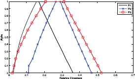 Figure 6:
The fuzzy RC of pi at t = 1
Alpha Alternatives p1 p2 p3 0 [0.025,0.362] [0.110,0.466] [0.019,0.522] 0.1 [0.032,0.342] [0.112,0.448] [0.030,0.502] 0.2 [0.040,0.321] [0.134,0.430] [0.039,0.481] 0.3 [0.048,0.301] [0.148,0.412] [0.052,0.460] 0.4 [0.057,0.281] [0.162,0.394] [0.068,0.438] 0.5 [0.069,0.261] [0.178,0.376] [0.087,0.417] 0.6 [0.083,0.242] [0.194,0.359] [0.107,0.395] 0.7 [0.099,0.223] [0.211,0.341] [0.130,0.373] 0.8 [0.117,0.204] [0.228,0.324] [0.154,0.352] 0.9 [0.135,0.186] [0.247,0.306] [0.180,0.331] 1 [0.155,0.169] [0.265,0.290] [0.207,0.310] Static rating 0.171 0.279 0.257 Static ranking 3 1 2 Dynamic rating E1(pi) 0.171 0.279 0.257 Dynamic ranking 3 1 2 Table 8.Alpha-level sets of fuzzy relative closenesses of the three alternatives at t = 1
Step 6. Computing dynamic rating
Since t = 1 and pi ∈ P1\ H0(i = 1,2,3), there is no historical available alternative. According to Eq. (33), the dynamic rating of each alternative, E1(pi), is equal to its corresponding static rating,
Since the dynamic rating, E1(pi), is equal to its corresponding static ratings,
While the alternative, p2, is selected and implemented to cope with the explosion for a while, the information related to the explosion is simultaneously changing because of its dynamic evolution. Hence, in order to make the emergency response pertinent and effective, the latest information about the explosion should be considered in the MAGEDM process. This is regarded as decision moment t = 2 in this case study.
4.1.2. Decision moment at t=2
Step 1. Framework definition
At decision moment, t = 2, one more expert, e4, is invited to participate in the decision process, that is, E2 = {e1, e2, e3, e4}. Furthermore, a new alternative, p4, and criterion, c4, are added, that is, P2 = {p1, p2, p3, p4} and C2 = {c1, c2, c3, c4}, which are given in Tables 9 and 10, respectively.
Alternatives Relationship with H1 Description p1 p1 ∈ P2 ∩ H1 Inform and evacuate citizens; meanwhile assign 10 fire squadrons, 300 fire fighters, and 40 fire engines to deal with the EE. p2 p2 ∈ P2 ∩ H1 Increase to 30 fire squadrons, 900 fire fighters, and 55 fire engines; at the same time, report the latest news to the citizens to avoid panic and riots. p3 p3 ∈ P2 ∩ H1 Ask the professional emergency rescue military for emergency rescue with more than 300 soldiers carrying specific equipment join in the rescue. p4 p4 ∈ P2 \ H1 Ask neighboring cities for their fire police to provide support; at the same time, fire police and military must collaborate to deal with the problems. Table 9.Description of alternatives at t = 2
Criteria Expression domain Description Social impacts (c4) S3, Sll It means the impacts on social development or people’s daily life, and so on, which are evaluated by experts by using linguistic terms si ∈ S3 = {None (N), Very Low (VL), Low (L), Medium (M), High (H), Very High (VH), Absolutely High (AH)}, and Sll generated by GH on the S3 (Same granularity with criterion c2). Table 10.Description of the added criterion c4 at t = 2
Step 2. Gathering information
The assessments,
Criteria c1 c2 c3 c4 [30,40] VLS [0.2,0.25] VL [50,60] LS [0.2,0.3] VL [40,60] LS [0.3,0.35] L [90,120] At least HS [0.55,0.65] H [40,50] VLS [0.25,0.35] VL [60,70] LS [0.3,0.35] VL [30,50] M [0.2,0.3] L [100,140] VHS [0.6,0.7] VH [30,50] LS [0.2,0.3] VL [40,50] LS [0.25,0.3] L [40,60] M [0.15,0.25] L [90,130] HS [0.5,0.7] VH [40,50] VLS [0.2,0.35] VL [60.70] VLS [0.2,0.3] VL [50,60] M [0.3,0.45] L [100,150] At least HS [0.65,0.8] VH Table 11.Assessments
Criteria c1 c2 c3 c4 HI MI LI HI VHI HI LI bt MI and HI HI MI LI HI VHI bt MI and HI LI HI Table 12.Criteria importance
Step 4. Aggregation process
Similar to decision moment, t = 1, to save space, only the aggregated results, X2 and
Aggregated results Criteria c1 c2 c3 c4 X2 x1j (0.030,0.035,0.048,0.050) (0,0.210,0.210,0.500) (0.020,0.021,0.031,0.035) (0,0.170,0.170,0.330) x2j (0.040,0.053,0.220,0.700) (0,0.290,0.290,0.500) (0.020,0.024,0.031,0.035) (0,0.210,0.210,0.500) x3j (0.030,0.040,0.058,0.060) (0.170,0.458,0.458,0.670) (0.015,0.024,0.034,0.045) (0.170,0.330,0.330,0.500) x4j (0.090,0.095,0.135,0.150) (0.500,0.805,0.805,1) (0.050,0.058,0.071,0.080) (0.500,0.790,0.790,1) (0.500,0.750,0.750,1) (0.330,0.543,0.585,0.840) (0.170,0.330,0.330,0.500) (0.350,0.628,0.670,0.840) Table 13.Aggregated results X2 and
Step 5. Computing static rating
Based on 11 alpha-levels, the results,
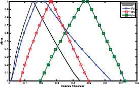 Figure 7:
The fuzzy RC of pi at t = 2
Alpha Alternatives p1 p2 p3 p4 0 [0.012,0.443] [0.015,0.639] [0.070,0.498] [0.197,0.724] 0.1 [0.023,0.403] [0.027,0.592] [0.084,0.474] [0.219,0.703] 0.2 [0.032,0.373] [0.041,0.545] [0.099,0.450] [0.243,0.682] 0.3 [0.040,0.343] [0.051,0.500] [0.115,0.427] [0.268,0.659] 0.4 [0.051,0.314] [0.063,0.455] [0.132,0.403] [0.294,0.636] 0.5 [0.063,0.285] [0.077,0.412] [0.151,0.380] [0.321,0.612] 0.6 [0.078,0.257] [0.094,0.371] [0.170,0.357] [0.349,0.589] 0.7 [0.093,0.230] [0.111,0.334] [0.191,0.334]r [0.377,0.564] 0.8 [0.110,0.203] [0.131,0.297] [0.212,0.312] [0.406,0.540] 0.9 [0.128,0.178] [0.151,0.261] [0.234,0.290] [0.435,0.516] 1 [0.146,0.153] [0.173,0.226] [0.257,0.269] [0.465,0.492] Static rating 0.179 0.253 0.269 0.468 Static ranking 4 3 2 1 Dynamic rating E2(pi) 0.319 0.461 0.457 0.468 Dynamic ranking 4 2 3 1 Table 14.Alpha-level sets of the fuzzy relative closenesses of the four alternatives at t = 2
Step 6. Computing dynamic rating
Due to pi ∈ P2 ∩ H1(i = 1,2,3), their dynamic ratings, E2(pi)(i = 1,2,3), should be calculated according to Eq. (33). In this case study, the associative aggregation operator utilized is the probabilistic sum function (a t-conorm exhibiting upward reinforcement, see Ref. 42 for details).
According to Definition 7, E2(p1) is computed as follows:
Since E1(p1) = 0.171 and
The dynamic rating, E2(pi), of each available alternative and the dynamic ranking of alternatives at t = 2 are given in Table 14 from rows 16 to 17, respectively.
According to Table 14, it can be seen that the dynamic ranking is different from the static one because the dynamic method considers the alternative behavior across the time. Therefore, based on the dynamic ranking, the DM can select the best alternative, p4, with the highest dynamic rating among P2 = {p1, p2, p3, p4} at decision moment, t = 2, to deal with the explosion. It can be seen that the best alternative has changed at t = 2 because the latest information about the explosion has been considered in the decision process.
While, the alternative, p4, is being carried out to deal with the explosion for a period, more information related to the explosion is collected along the time. The latest collected information should be also considered in the MAGEDM process. It is regarded as decision moment, t = 3.
4.1.3. Decision moment at t=3
Step 1. Framework definition
At decision moment, t = 3, alternative, p1, is removed due to its ineffectiveness; meanwhile a new criterion, c5, and one new alternative, p5, are added, that is, C3 = {c1, c2, c3, c4, c5}, P3 = {p2, p3, p4, p5}, which are given in Tables 15 and 16, respectively.
Criteria Expression domain Description Cost of alternative (c5) I It means the cost of alternative, pi, (i = 2, 3, 4, 5), including all the direct and indirect expenses in domain [0,100] (in million RMB). Table 15.Description of the added criterion c5 at t = 3
Alternatives Relationship with H2 Description p2 p2 ∈ P3 ∩ H2 Increase to 30 fire squadrons, 900 fire fighters, and 55 fire engines; at the same time, report the latest news to the citizens to avoid panic and riots. p3 p3 ∈ P3 ∩ H2 Ask the professional emergency rescue military for emergency rescue with more than 300 soldiers carryinh specific equipment join in the rescue. p4 p4 ∈ P3 ∩ H2 Ask neighbor cities for their fire police in order to provide support; at the same time, fire police and military must collaborate to deal with the problems. p5 p5 ∈ P3 \ H2 Block the boundary of the explosion areas; let the material in the explosion areas burn down. Table 16.Description of alternatives at t = 3
Step 2. Gathering information
The criteria importance,
Criteria c1 c2 c3 c4 c5 HI MI LI HI MI VHI HI LI HI MI VHI LI VLI MI VLI HI MI LI MI VLI Table 17.Criteria importance
Criteria c1 c2 c3 c4 c5 [80,90] M [0.3,0.4] L [30,50] [50,70] M [0.25,0.35] M [40,60] [90,120] bt M and HS [0.35,0.45] H [70,80] [70,100] VHS [0.4,0.5] VH [25,45] [60,80] LS [0.15,0.25] VL [50,60] [70,90] LS [0.3,0.4] L [40,55] [90,110] At most M [0.4,0.5] M [60,80] [50,70] HS [0.25,0.4] VH [35,50] [40,50] VLS [0.2,0.25] L [40,60] [60,75] M [0.15,0.2] L [30,50] [80,100] M [0.4,0.45] H [70,90] [30,45] VHS [0.1,0.25] VH [25,45] [45,65] LS [0.35,0.4] VL [35,55] [40,60] bt LS and M [0.5,0.55] L [30,45] [70,80] M [0.6,0.7] M [60,75] [30,50] HS [0.3,0.5] H [30,35] Table 18.Assessments
Step 4. Aggregation process
To save space, similar to t = 2, only the aggregated results, X3 and
Aggregated results Criteria c1 c2 c3 c4 c5 X3 x2j (0.040,0.056,0.071,0.090) (0,0.333,0.333,0.670) (0.015,0.025,0.033,0.040) (0,0.250,0.250,0.500) (0.300,0.388,0.563,0.600) x3j (0.040,0.055,0.074,0.090) (0.170,0.418,0.458,0.670) (0.015,0.030,0.038,0.055) (0.170,0.373,0.373,0.670) (0.300,0.350,0.525,0.600) x4j (0.070,0.083,0.103,0.120) (0,0.375,0.508,0.840) (0.035,0.044,0.053,0.070) (0.330,0.585,0.585,0.830) (0.600,0.650,0.813,0.900) x5j (0.030,0.045,0.066,0.100) (0.500,0.750,0.750,1) (0.010,0.026,0.041,0.050) (0.500,0.790,0.833,1) (0.250,0.288,0.438,0.500) (0.500,0.750,0.750,1) (0.170,0.500,0.500,0.830) (0,0.290,0.290,0.500) (0.330,0.585,0.585,0.830) (0,0.335,0.335,0.670) Table 19.Aggregated results X3 and
Step 5. Computing static rating
Based on 11 alpha-levels, the fuzzy RC,
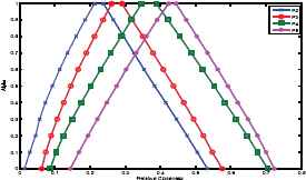 Fig. 8.
The fuzzy relative closeness of pi at t = 3
Alpha Alternatives p2 p3 p4 p5 0 [0.015,0.534] [0.063,0.575] [0.088,0.704] [0.145,0.723] 0.1 [0.030,0.505] [0.075,0.548] [0.104,0.675] [0.169,0.700] 0.2 [0.046,0.475] [0.090,0.522] [0.125,0.646] [0.194,0.675] 0.3 [0.058,0.445] [0.107,0.494] [0.149,0.615] [0.221,0.648] 0.4 [0.074,0.415] [0.126,0.466] [0.176,0.584] [0.248,0.620] 0.5 [0.093,0.384] [0.146,0.437] [0.203,0.552] [0.276,0.592] 0.6 [0.114,0.354] [0.167,0.408] [0.231,0.520] [0.303,0.562] 0.7 [0.137,0.324] [0.190,0.379] [0.260,0.487] [0.331,0.533] 0.8 [0.161,0.295] [0.213,0.350] [0.288,0.454] [0.361,0.503] 0.9 [0.186,0.267] [0.237,0.320] [0.317,0.421] [0.391,0.473] 1 [0.213,0.239] [0.262,0.291] [0.347,0.388] [0.423,0.444] Static rating 0.244 0.294 0.379 0.433 Static ranking 4 3 2 1 Dynamic rating E3(pi) 0.593 0.617 0.670 0.433 Dynamic ranking 3 2 1 4 Table 20.Alpha-level sets of the fuzzy relative closenesses of the four alternatives at t = 3
Step 6. Computing dynamic rating
Similar to t = 2, the dynamic rating, E3(pi), and the dynamic ranking of alternatives at t = 3 are given in Table 20 from rows 16 to 17, respectively. Again, dynamic and static rankings are different. Therefore, based on the dynamic ranking of the four alternatives in Table 20, p4 is the best one with the highest dynamic rating among P3 = {p2, p3, p4, p5} at t = 3 to cope with the explosion.
It can be seen that the best alternative, p4, at t = 3, is consistent with the best one at t = 2. This interesting phenomenon can be explained by the fact that the dynamic rating here consists of not only each alternative’s performance at current stage, but also at previous stage.
To save space, only three different decision moments have been conducted in this case study. In real world problems, the proposed dynamic MAGEDM method can be applied for more than three decision moments until the problems are solved.
4.2. Comparison with other approaches
To further demonstrate the feasibility and validity of the proposed dynamic MAGEDM method, a comparison with the approach introduced by Campanella et al. 4 is carried out, along with their discussions.
- 1)
A brief summary of current dynamic EDM methods is provided to highlight the advantages of our proposal.
- 2)
A current dynamic MADM approach 4 is utilized for the comparison with our proposed method.
4.2.1. Comparison with current dynamic EDM methods
Due to the fact that there is no any existing MAGEDM approach to deal with dynamic evolution of EEs considering updated information (alternative, criteria and experts) and experts’ hesitation, some characteristics have been studied to highlight the advantages of our proposal in comparison with other approaches 13,29,31,40 (see Table 21).
| Literature | Type of decision | Perspective of dynamic | Hesitant information |
|---|---|---|---|
| Refs. 13, 29 | Individual DM | Time changes and executive effect of alternative, without updated information (alternative, criteria) | No |
| Refs. 31 | Individual DM | Time changes and dynamic reference points, without updated information (alternative, criteria) | No |
| Refs. 40 | Group decision | Time changes and similarity between predicated scenario and historical scenario, without updated information (alternative, criteria, expert) | No |
| Our proposal | Group decision | Time changes with updated information (alternative, criteria, experts) | Yes |
Comparison with current dynamic EDM methods
According to Table 21, we can see that current dynamic EDM methods are mainly focused on the perspective of time changes. However, our proposal deals with the dynamic evolution of EEs not only from the perspective of time, but also considering the updated information (alternative, criteria, and experts) along with the time and development of EEs. Therefore, the decision processes are more close to real world situations than the current dynamic EDM methods.
Furthermore, our proposal considers experts’ hesitation due to lack of information and time pressure, which is inevitable in EDM problems.
4.2.2. Comparison with a current dynamic MADM method
To make a comparison with the recent dynamic MADM method proposed by Campanella et al. 4, the aggregated results, Xt and
| Decision moment | Criteria | |||||
|---|---|---|---|---|---|---|
| c1 | c2 | c3 | c4 | c5 | ||
| t = 1 | p1 | 0.058 | 0.268 | 0.031 | - | - |
| p2 | 0.094 | 0.500 | 0.046 | - | - | |
| p3 | 0.042 | 0.466 | 0.026 | - | - | |
| weights | 0.832 | 0.624 | 0.268 | - | - | |
| t = 2 | p1 | 0.041 | 0.223 | 0.027 | 0.168 | - |
| p2 | 0.214 | 0.277 | 0.028 | 0.223 | - | |
| p3 | 0.048 | 0.445 | 0.029 | 0.332 | - | |
| p4 | 0.117 | 0.787 | 0.065 | 0.777 | - | |
| weights | 0.750 | 0.571 | 0.332 | 0.631 | - | |
| t = 3 | p2 | 0.064 | 0.333 | 0.028 | 0.250 | 0.467 |
| p3 | 0.065 | 0.432 | 0.034 | 0.388 | 0.442 | |
| p4 | 0.093 | 0.434 | 0.050 | 0.583 | 0.738 | |
| p5 | 0.059 | 0.750 | 0.033 | 0.791 | 0.367 | |
| weights | 0.750 | 0.500 | 0.277 | 0.583 | 0.335 | |
- means the criteria unavailable in specifical decision moment
Defuzzied values of Xt and
As the sum of defuzzied criteria weights in Table 22 at each decision moment is greater than 1, and it must be equal to 1, it is necessary to normalize the weights. The normalized criteria weights at each decision moment are given in Table 23.
| Decision Moment | Normalized criteria weights | ||||
|---|---|---|---|---|---|
| c1 | c2 | c3 | c4 | c5 | |
| t = 1 | 0.483 | 0.362 | 0.155 | - | - |
| t = 2 | 0.329 | 0.250 | 0.145 | 0.276 | - |
| t = 3 | 0.307 | 0.204 | 0.113 | 0.239 | 0.137 |
- means the criteria unavailable in specifical decision moment
Normalized criteria weights at each decision moment
Based on Tables 22 and 23, static and dynamic ratings for each alternative at different decision moments are computed with the weighted mean operator and probabilistic sum operator (e.g., associative) according to the method presented in Ref. 4. The results are given in Table 24.
| Decision moment | Alternatives | |||||
|---|---|---|---|---|---|---|
| p1 | p2 | p3 | p4 | p5 | ||
| t = 1 | Static rating | 0.130 | 0.144 | 0.237 | - | - |
| Static ranking | 3 | 2 | 1 | |||
| Dynamic rating | 0.130 | 0.144 | 0.237 | - | - | |
| Dynamic ranking | 3 | 2 | 1 | - | - | |
| t = 2 | Static rating | 0.120 | 0.205 | 0.223 | 0.459 | - |
| Static ranking | 4 | 3 | 2 | 1 | ||
| Dynamic rating | 0.234 | 0.319 | 0.407 | 0.459 | - | |
| Dynamic ranking | 4 | 3 | 2 | 1 | - | |
| t = 3 | Static rating | - | 0.215 | 0.265 | 0.363 | 0.414 |
| Static ranking | - | 4 | 3 | 2 | 1 | |
| Dynamic rating | - | 0.466 | 0.564 | 0.655 | 0.414 | |
| Dynamic ranking | - | 3 | 2 | 1 | 4 | |
- means the alternative unavailable in specifical decision moment
The results obtained by the method in Ref. 4
For the sake of clarity, an example, the static rating of p1 at t = 1 in Table 24, can be computed as below:
The dynamic rating of p1 at t = 2 can be calculated based on its static rating (0.120) at t = 2, and its dynamic rating (0.130) at t = 1, as shown below:
From Table 24, it can be seen that, although the method in Ref. 4 leads to the same best alternatives at different decision moments (t = 2,3), it is obvious that the values obtained by the method in Ref. 4 are significantly lower than those obtained by our proposed method at each decision moment. This is because our proposal deals with uncertain information, including experts’ hesitation. Additionally, the computation process retains as much information as possible. Therefore, the proposed method shows its validity and feasibility through the comparison.
4.2.3 Discussions
To overcome the limitations pointed out in section 1, this paper proposes a dynamic MAGEDM method to deal with the dynamic evolution of EEs and uncertain information including experts’ hesitation. A case study and comparisons with current approaches have been conducted to demonstrate the novelty and validity of the proposed dynamic MAGEDM method.
Compared to existing MAGEDM approaches 11,16,30,35,36,37,38, the advantages of the proposed dynamic MAGEDM method are as follows:
- 1)
The proposed dynamic MAGEDM method considers the dynamic evolution feature of EEs, which is a crucial factor in real world problems; it fully takes into account the updated information across the time and the development of EEs. The proposed method is close to the real-world situations and easy to understand. This is the significant difference between our proposal and other versions 13,29, wherein the alternatives and criteria are fixed without considering the updated information along the time.
- 2)
Hesitancy is a quite normal behavior in human beings daily life particularly in uncertain environment. Experts involved in MAGEDM problems featured by lack of information and time pressure might hesitate among several values when they provide their opinions, however, such a practical issue is neglected in existing MAGEDM approaches 11,16,30,35,36,37,38. To fill the gap in current MAGEDM approaches, the proposed method has taken into account the experts’ hesitation by using complex linguistic expressions based on HFLTS.
- 3)
To keep the uncertain and hesitant information provided by experts as much as possible, a fuzzy TOPSIS method based on alpha-level sets is utilized to obtain the static ratings of alternatives at each decision moment, which can provide much more information for each alternative and is suitable for the problems defined in fuzzy environment.
5. Conclusion and future works
Dynamic evolution and uncertain information are the outstanding features of EEs, they are the key factors in the process of dealing with the EEs successfully. Information plays a crucial part in all different types of decision problems no exception for MAGEDM problems. Due to the dynamic evolution of EEs, the information is updating along with the time and the development of EEs. However, the dynamic methods in current EDM approaches are mainly focused on changeable time; they neglect information changes along with the evolution of EEs. The information is usually uncertain in MAGEDM problems—particularly in the early occurrence stage—in such a fuzzy environment that experts might hesitate about their assessments. However, this important issue is not considered in current MAGEDM problems. Thus, this paper proposes a dynamic MAGEDM method that considers not only the dynamic evolution of EEs, including the updated information (alternatives, criteria, and experts), but also the experts’ hesitation. A fuzzy TOPSIS method based on alpha-level sets is applied to obtain the static ratings of available alternatives, which deals with fuzzy information across the decision process, and is suitable for the problems defined in fuzzy environments. Comparisons with other approaches and related discussions have been provided to illustrate the novelty and advantages of our proposal.
Future research could investigate use of decision support systems with big data based on computer science and the Internet.
Acknowledgment
The authors would like to thank all the anonymous reviewers and the Editor-in-Chief for their valuable time and constructive suggestions and comments to improve our paper. This work was partly supported by the Young Doctoral Dissertation Project of Social Science Planning Project of Fujian Province (Project No. FJ2016C202), National Natural Science Foundation of China (Project No. 71371053, 61773123), Spanish National Research Project (Project No. TIN2015-66524-P), and Spanish Ministry of Economy and Finance Postdoctoral Fellow (IJCI-2015-23715).
Footnotes
Background Information. http://www.safehoo.com/Case/Case/Blow/201602/428723.shtml
References
Cite this article
TY  - JOUR
AU  - Liang Wang
AU  - Rosa M. Rodríguez
AU  - Ying-Ming Wang
PY  - 2018
DA  - 2018/01/01
TI  - A dynamic multi-attribute group emergency decision making method considering experts’ hesitation
JO  - International Journal of Computational Intelligence Systems
SP  - 163
EP  - 182
VL  - 11
IS  - 1
SN  - 1875-6883
UR  - https://doi.org/10.2991/ijcis.11.1.13
DO  - 10.2991/ijcis.11.1.13
ID  - Wang2018
ER  -