
Particle Swarm Optimization and harmony search based clustering and routing in Wireless Sensor Networks
- DOI
- 10.2991/ijcis.10.1.84How to use a DOI?
- Keywords
- Particle swarm optimisation; clustering; harmony search; routing algorithm; network lifetime
- Abstract
Wireless Sensor Networks (WSN) has the disadvantage of limited and non-rechargeable energy resource in WSN creates a challenge and led to development of various clustering and routing algorithms. The paper proposes an approach for improving network lifetime by using Particle swarm optimization based clustering and Harmony Search based routing in WSN. So in this paper, global optimal cluster head are selected and Gateway nodes are introduced to decrease the energy consumption of the CH while sending aggregated data to the Base station (BS). Next, the harmony search algorithm based Local Search strategy finds best routing path for gateway nodes to the Base Station. Finally, the proposed algorithm is presented.
- Copyright
- © 2017, the Authors. Published by Atlantis Press.
- Open Access
- This is an open access article under the CC BY-NC license (http://creativecommons.org/licences/by-nc/4.0/).
1. Introduction
A wireless sensor network (WSN) comprise of hundreds of low cost, low-power portable sensor nodes deployed in close proximity to a physical phenomenon which can be use in a numerous applications such as national security, environment monitoring, military reconnaissance, traffic control. Nevertheless, any real time application that requires data gathering from a geographically localized region. Each node in a WSN must send data to a special node called Base Station (BS), which is placed far away from the sensor network. These sensors in a network have limited battery powered energy resource; thus energy efficiency is a very important criteria for designing the network topology and routing path. Several metric can be considered to measure the performance of WSN includes network scalability, network lifetime, routing overhead, energy consumption1. The clustering has been proven an effective means to increasing scalability and the lifetime of WSNs1. In clustering scheme, the complete network of sensors divided into graphically confined regions called clusters. Each cluster contains a cluster head, which is either pre-defined special purpose node or selected from one of the sensor nodes of a cluster using appropriate algorithm. This cluster head is used to receive data from the rest of the nodes of belonging cluster in a TDMA fashion1 (or any of the other multiple channel access protocols). After removing the redundancy by aggregate the data, the cluster head further send these data to BS. However, sending the data to BS from one sensor node may not always be possible due to the fact that BS may be beyond the transmission range of that sensor node. The multi-hop techniques can be a solution to overcome this problem by sending the data to BS via a series of intermediate sensor nodes. Additionally, an efficient multi-hop routing algorithm can also increase the network lifetime.
The distance from the BS is a crucial factor for energy consumption among cluster heads and gets imbalanced due to the distance mismatch. The cluster heads farther away from the BS need to transmit data to a longer distance in single-hop networks. However in multi-hop networks, cluster heads closer to BS are used as data forwarding nodes and thus transmit more times than it would in a single-hop network. This creates energy depleted nodes in close proximity, usually termed as Energy Hole Problem18. The energy aware clustering and routing approaches can be adopted to overcome above problem. Relay node can be used which acts as intermediary between CH and base station (BS) to reduce traffic load between the CH and BS19.
In the present paper, a novel approach is proposed which make use of two optimization techniques at different phases. The first objective of the proposed scheme is to select a cluster head with Particle Swarm Optimization. A gateway node is introduced between the sink and the cluster head to achieve second objective of routing using Particle Swarm optimization. These gateway nodes are used to reduce the energy consumption of the CH while sending aggregated data to the base station21. The cluster head first transfers the aggregated data to the gateway node provided the distance between the cluster head and sink is long which further transfers to the sink. The selection of the gateway nodes or the base station is solo based on the close distance with cluster head for aggregated data transfer. As a consequence, cluster head can achieve better energy efficiency due to less energy consumption together with increase in its life time.
2. Related Work
A wireless sensor networks (WSNs) have become an important technology in a wide variety of application due to its low cost, small size, and self-organization. It has now become an important technology in recent years. The energy efficiency of routing protocols in WSN still remains an open challenge for research community1. There are several clustering and routing protocols were proposed in the literature for sensor networks2–4, for generating stable clusters and energy efficient routing path as a main objective.
In the recent research many clustering and routing algorithms is formulated as optimization problems16–17. The Particle Swarm optimization (PSO) is a approach to improve network lifetime .The algorithm propose to construct the path and distribute the routing data through the Cluster Heads or gateway node close to the Base Station, which maximizes the network timeline.
An energy aware selection of CH using PSO is called PSO-C6, which is based on the ratio of total initial energy of all nodes to the total present energy of all CHs and an average distance between the CHs. However, the sink distance is not accounted for the communication between cluster heads (CHs) and Base Station, which is important to minimize the energy consumed by the network. Moreover, the assignment of non-CH sensor nodes to the nearest CH in the cluster formation phase, can possibly lead to the energy inefficiency in the network, which lowers the lifetime of the network. Another, energy aware novel CH selection algorithm5 using PSO brings the whole latest fitness function based on the remaining energy of all the nodes, node density and the distance. However, it ignores the phase where the cluster is formed and can lead to lots of inefficient energy into the network. Furthermore, leaving the cluster formation in the algorithm can impact on the consumption of energy of the network. The10–13 published literature; have proposed few protocols based on application for WSNs such as, cloud based body sensor network ambient intelligence with other network problems. The methods for energy efficient clustering based on recent variable population based chemo-inspired approach has been proposed7 Wireless Network called as a novel chemical reaction optimization (nCRO). It prolongs the network lifetime significantly. Moreover, the CHs interact directly to the BS, which may or may not be feasible for large scale network. An algorithm based on nCRO approach14 for addressing the scalability problem in reference7 , has been proposed, which solves the hot spot problem in wireless sensor networks to some extent but ignores the fault tolerance and issues related to delaying in WSN. Algorithm based on PSO for time sensitive applications, has been proposed15, which has accounted for efficiency related to energy and elongates the network lifetime.
Energy-efficient ant-based routing algorithm (EEABR), in which the basic idea is based on the Ant Colony Optimization (ACO) routing16. Improved harmony search based energy-efficient routing algorithm (IHSBBER) is routing algorithm based on harmony search algorithm is proposed. The disadvantages of limited and non-rechargeable energy resource in WSN create a major challenge of designing of the energy efficient wireless sensor networks. It is expected to balance the energy consumption of network for routing, so as to prolong the network lifetime17.
2.1. Particle Swarm Optimization
Particle swarm optimization (PSO) is inspired by nature. It is based on swarm intelligence, modeled after noticing the activity of a flock of birds, i.e., their ability to exploit and explore the search space for their living. Particle Swarm Optimization is a very simple algorithm. Over various iterations, the variables adjust themselves closest to the member whose value is close to the solution. The algorithm based on PSO consists of a pre- defined particle number say NP, known as a swarm. Every particle gives a potential solution. A particle Pi, 1 ≤ i ≤ Np has position Xi, d and velocity Vi,d, 1 ≤ d ≤ D in the dth dimension of the search space. The dimension D is similar for all particles. A fitness function evaluates each particle for verifying the superiority of the solution. Each particle keeps an eye on its dimensions in the problem space which are associated with solution that is its best fitness value which it has gained so far. This value is called best. Another “best” value that is traced by the PSO is the best value, obtained so far by any particle in the neighbors of the particle. This location is called Lbest when a particle takes all the nodes as its topological neighbors, the best value is a global best and is called gbest.
To reach the global best solution, gbest, it uses its personal and global best to update the velocity Vi,d and position Xi,d using the following equations.
2.2. Harmony Search Algorithm
The Harmonic Search Algorithm has a very simple concept and employs the use of very few parameters yet has a very strong global search capacity. The classical Harmony Search algorithm comprises of the following main steps.
- 1.
Initializing the optimization problem and algorithm parameters.
- 2.
Initializing the Harmony Memory (HM).
- 3.
Improvisation of a new harmony.
- 4.
Updating the Harmonic Memory.
- 5.
Repeating step (3) and step (4) until the termination criterion is satisfied.
The Harmony Memory designed to accommodate harmonies of the same size can’t be used for routing for WSNs, as in it the number of sensor nodes in path is uncertain. Thus, the size of the harmony in HM may be different. Therefore, the classical HS algorithm can’t be directly used to solve routing problem of WSNs. Several improvements to the classical approach have been made to make it suitable for use in WSNs.
2.2.1 Improvements in harmony search algorithm to make it suitable for WSN
In WSN routing, a harmony represents a forwarding path that consists of the sensor nodes that will be present in it. The first node is source node and the last node is sink node. Thus we can see that the size of the harmonies will be different as in different scenarios, the no of nodes in the path will be different. Thus the encoding of the harmony memory is changed so as to accommodate different sized values for different paths.
The Harmonic Search algorithm uses a parameter known as Harmonic Memory Considering Rate (HMCR) that has a static value anywhere between 0 and 1. The HMCR helps the search algorithm to find the optimum path for given input. In the IHSBEER algorithm, an adaptive HMCR is used whose value alters dynamically with the no of iterations so as to find the global optimum solution for the given input. A new objective function, which considers both, the energy consumption of the network as well as the length of the path so as to find a solution that balances both of them, is employed. This function makes sure that the most efficient path is found.
2.2.2. IHSBEER description
The IHSBEER algorithm consists of the following steps:
- 1.
Encoding of the harmony memory.
Here the harmony memory is encoded so as to accommodate harmonies of different sizes. This is shown below:
Here ‘s’ is the source node, ‘d’ is the sink node. Xi, i.e., (s, xi,2, …, xi,j, …, d), is the ith harmony, which represents the ith forwarding path from source node and the sink node. This encoding has made a tremendous contribution in making the Harmonic Search Algorithm suitable for the WSN Routing problem.
- 2.
Initialization of Harmony Memory
The Harmonic Memory is initialized using the roulette wheel selection method. The probability P(i,j) of node i selecting node j as the next hop is given by the equation
Here:
- hk =
hop count of node k to the sink node
- hj =
hop count of node j to the sink node
- Ni =
Set of neighboring nodes of node I, except for the nodes that are already present in the current forwarding path.
- C(Ni) =
Capacity of the set Ni
The nodes closer to the sink node and in the communication range of the current node are more likely to become next hop. Thus a good initial harmony can be generated which eases the further optimization process.
Roulette Wheel Selection Method
A random number R between 0 and 1 is generated. The R is used to subtract the probability P of the first node in Ni. If the value of subtraction is negative, choose the first node in Ni as the next hop of node i else the value of subtraction is used to subtract the probability P of the second node in Ni. Then, whether the value of second subtraction is positive or negative, is determined. If it is negative, second node in Ni is selected as the next hop of node i. Otherwise, this operation will continue till the value of subtraction is negative and the corresponding node in Niis selected as the next hop of node i.
- 3.
Improvisation of a new harmony. (Generation of a new path)
In this step, the Harmony Search Algorithm is applied to design routing approach for WSNs.
Supposing X′ = (s, x2′ , …, xi′ , …, d) is a new harmony, the element xi′ is selected by memory considerations according to the requirements of routing for WSN,
Here:
- HMCR=
Harmony Memory Consideration Rate
- N(x′i-1)=
Set of neighboring nodes, except for the nodes that are already present in the current forwarding path.
- P1=
A random no between 0 and 1.
For the new harmony, X′ = (s, x′2 , …, x′i , …, d), if x′i is selected from HM, the adjusting decision-making for x′i is done as follows: If P2 is smaller than PAR, x′i needs to be adjusted. Otherwise, it remains unchanged. PAR is the Pitch Adjusting Rate varying from 0 to 1, and P2 is a random number between 0 and 1.
Adaptive HMCR
If the HMCR keeps a small static value over the iterations, it will lose its local search ability with time. Similarly if it keeps a large static value, it’ll only find the local optimum result. Therefore an adaptive value of the HMCR is required. The value of the HMCR isn’t kept static and changes according to the exponential rule:
Here:
- HMCR(gn)=
Value of HMCR in gth generation
- HMCRmax=
Maximum HMCR value
- HMCRmin=
Minimum HMCR value
- NI=
Maximum no of iterations
- 4.
Objective Function
Radio model is used, where the transmitter or receiver circuitry dissipates. Therefore, to transmit or receive the radio expends:
And to receive this message the radio expends:
Suppose that a path X=(s, x2, …, xi, …, d) contains L nodes, i.e., the number of elements in X is L, the energy consumption of transmitting a k-bits message along this path is calculated as follow:
Where
Next, a new objective function to balance the length of the path and the energy consumption is proposed as:
Here:
- Emin=
Residual energy of the node having minimum residual energy in path X
- EAvg=
Average residual energy of all the nodes in path X
3. Proposed Methodology
In this section Particle swarm optimisation based clustering and harmony search based routing algorithm is proposed. So in this paper, global optimal cluster head (collect data from all member nodes) and gateway nodes are selected using Particle swarm optimisation based clustering. To compare the performance of the proposed approach, two metric are used viz. Average residual energy and network lifetime. Next, the harmony search algorithm based Local Search strategy finds different routing paths for each gateway nodes to the BS. Gateway node (act as a source node in harmony search) which have best route to the base station, for routing data to the base station. Finally, the proposed algorithm is presented.
3.1. Particle Swarm Optimisation Based Clustering
- 1.
Initialize all node with constant value of energy and Deploy them in a specific area.
- 2.
Randomly assign 10% of n nodes as cluster heads.
- 3.
Find the nearest cluster head for all the normal nodes
- 3.1
For i : 1 to n (total number of nodes)
- 3.1.1
Initialize minimum_distance with dis (distance of node i from sink)
- 3.1.2
For j: 1 to m(total number of cluster heads)
distance = dij (distance from node i to CH j)
if(minimum_distance > distance)
minimum_distance = distance
cluster.id = j
end if
End For
- 3.1.3
Calculate the minimum average intra cluster distance and sink distance of all CHs (f1)
- 4.
Calculate the parameter to maximize the total energy of CHs using (5)
- 5.
Calculate Fitness for each node
For i : 1 to n
Fitness(i) = f1 × α1 + f2 × (1- α1)
Pbesti = Fitness(i)
End For
- 6.
Initialize velocity of each node with zero.
- 7.
Assign the lowest value of pbest among all pbest to gbest.
- 8.
For r : 1 to total number of rounds
- 9
Find the velocity and position of each node using PSO algorithm by equation (1) and (2)
- 9.1
Repeat step 3 for finding nearest cluster head for all the normal nodes.
- 9.2
Repeat step 4 and 5 for calculating f1 and f2.
- 9.3
Calculate Fitness and update pbest
For i : 1 to n
Fitness(i) = f1 × α1 + f2 × (1- α1)
if(Fitness(i) <= Pbesti)
Pbesti = Fitness(i)
end if
End For
- 9.4
Repeat step 8 to calculate gbest
- 9.5
Mark 10% nodes with minimum pbest values as the new CHs and all the other nodes as normal
Nodes
End For
3.2 Harmony Search Based Routing Process
In this section when we get the optimal cluster heads (CHs) from the PSO clustering algorithm, as an input to next algorithm for routing data packet to the sink node. A basic implementation of the routing process is as follows.
- b1)
A subset of CH is selected as a gateway node, which act as a source node in harmony search based routing. The gateway node should not be near to sink node. A subset of CHs which are minimum distance (threshold distance) away from the sink node are taken as gateway node. While the CHs near the sink can directly send their data to Sink.
- b2)
Cluster heads send data to the nearby gateway node. Gateway node act as a source node in harmony search algorithm.
- b3)
Each gateway node sends the packet containing information about the node to the sink node. The sink node will execute the routing algorithm to find the forwarding path.
- b4)
The forwarding path is stored in memory and its residual energy gets added to the packet. Then the gateway node will transmit the packet to next hop according to the forwarding path.
- b5)
The next hop has received the packet, it adds its residual energy, and deletes the node, which has been visited, from the forwarding path.
- b6)
The packet send to the next hop according to the forwarding path. This step repeated until the packet has been received by the sink node.
- b7)
Sink node receives the packet, it processes and sends to the observer then, updates the residual energy of those nodes in the packet.
- b8)
The sink node transmits the packet containing forwarding path to each sensor node in single hop at regular interval. If any new forwarding path is similar to the previous path stored in the node, the sink node does not send a packet to the node.
4. Results and Discussion
This section presents the simulation results of the proposed algorithm. Different network scenarios were considered, number of nodes varied from 100 to 400 with 10 percent of cluster head are taken for each scenario. And the simulated area is also varied from 200 × 200 m2 to 400 × 400 m2 for all nodes taken into consideration. For each network scenario two metrics were used to compare the performance of proposed algorithm. Average Residual energy for all nodes and network lifetime is number of iterations that the networks have sustained until any nodes run out of energy. Following are the simulation parameters taken for Particle swarm optimisation based clustering harmony search based routing algorithm given in Table 2.The simulation parameters are taken similar to the papers [15, 17, 22, 23, and 24] .
Table 1 shows the no of times data transmission takes place before a node in the path falls below the threshold energy level and the transmission stops. When the area of the sensor field is kept 200×200 m2 , we can see from Fig 1. that the number of iterations that network have sustained until any node exhausted for the proposed algorithm (PSO-HSA) which is always greater than that of the EEABR and IHSBBER algorithm in different network scenarios. The Standard deviation of residual energy is calculated as reported in paper17.
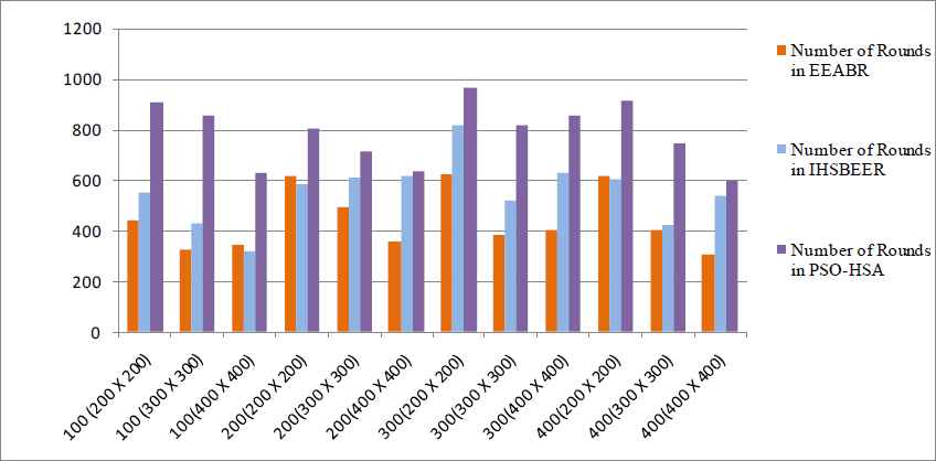
Network lifetime vs number of nodes (Sensor field area)
| No. of Nodes | Area of Sensor Field | No. of iterations in EEABR | No. of iterations in IHSBEER | No. of iterations in PSO-HSA |
|---|---|---|---|---|
| 100 | 200 × 200 | 441 | 556 | 910 |
| 100 | 300 × 300 | 327 | 431 | 860 |
| 100 | 400 × 400 | 344 | 320 | 630 |
| 200 | 200 × 200 | 618 | 586 | 810 |
| 200 | 300 × 300 | 496 | 611 | 720 |
| 200 | 400 × 400 | 356 | 622 | 640 |
| 300 | 200 × 200 | 624 | 822 | 970 |
| 300 | 300 × 300 | 386 | 523 | 820 |
| 300 | 400 × 400 | 403 | 632 | 860 |
| 400 | 200 × 200 | 618 | 606 | 920 |
| 400 | 300 × 300 | 404 | 427 | 750 |
| 400 | 400 × 400 | 308 | 541 | 600 |
No of iterations before reaching threshold energy
| Parameter | Values | |
|---|---|---|
| Deploying area | 200 × 200 m2 , 300 × 300 m2 , 400 × 400 m2 | |
| Sensor node’s energy | 2 J | |
| Number of sensor nodes | 100,200,300,400 | |
| Location of BS | (200,200) for 200 × 200 m2 , (300,300) for 300 × 300 m2, (400,400) for 400 × 400 m2 | |
| Percentage of CHs | 10 % | |
| Eelec | 50 nJ/bit | |
| Efs | 10 pJ/bit/m2 | |
| Emp | 0.0013 pJ/bit/m4 | |
| d0 | Sqrt(Efs/Emp) m | |
| Packet length | 4000 bits | |
| Number of particles | 30 | |
| Number of iterations | 100 | |
| C1 | 2 | |
| C2 | 2 | |
| χ1 | .5 | |
| χ2 | .7 | |
| α1 | .3 | |
| w | .7 | |
| D | 10-40 | |
| Vmax | 200 | |
| Communication radius | 150 m | |
| HMS | 5 | |
| HMCR in IHSBEER, PSO-HSA | HMCRmin = 0.2, HMCRmax = 0.9 |
|
| Evaluation times | 500 | |
| Initial pheromone | 1 | |
| α, β, ρ | α = 1, β = 5, ρ = 0.0 |
Simulation Parameters
In Fig 2 the Standard deviation of residual energy is calculated as reported in paper17. More the value of standard deviation of nodes residual energy signify the energy is not averagely consumed in the network whereas smaller standard deviation means better results because it signify the balanced energy consumption. The three algorithms have almost equal performance in balancing the energy consumption of networks. The reason may be because of all the events occur in the same place and all the packets are sent out from the same source node for the three algorithms in each scenario. The metrics used to compare the performance are as follows:
- (1)
Average residual energy defined as the average residual energy (remaining energy at each iteration) of all nodes.
- (2)
Standard deviation of residual energy represents the standard deviation of residual energy levels on all nodes.
- (3)
Network lifetime defined as the duration from the start of the network until any node runs out of energy.
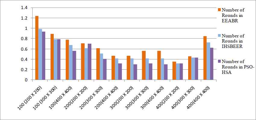
Standard deviation of residual energy vs number of nodes (Sensor field area)
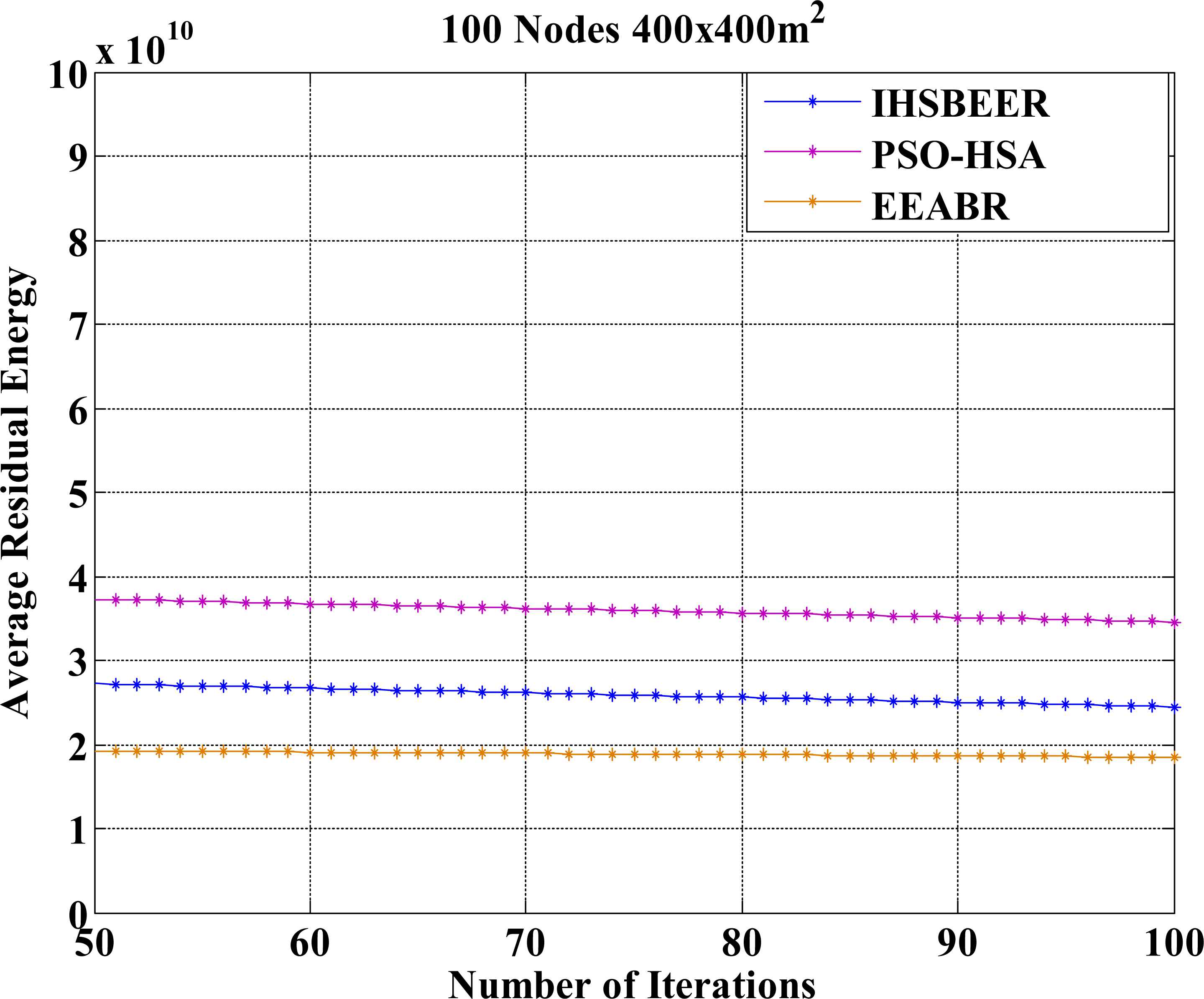
In Fig. 3 and Fig 4 represents the number of average residual energy of all nodes is much higher than the existing algorithms after certain rounds. This is because of the introduction of Gateway node. Fig 3 shows the result for 100 node in 200×200 m2 area with 10 clusters. CHs send data to GN in order to send data to BS. GN should not be less than Dth (threshold distance) because if CH is very near to BS , it can directly send data to BS. GN act as a Source node in HSA which creates the best path in order to send data to BS.
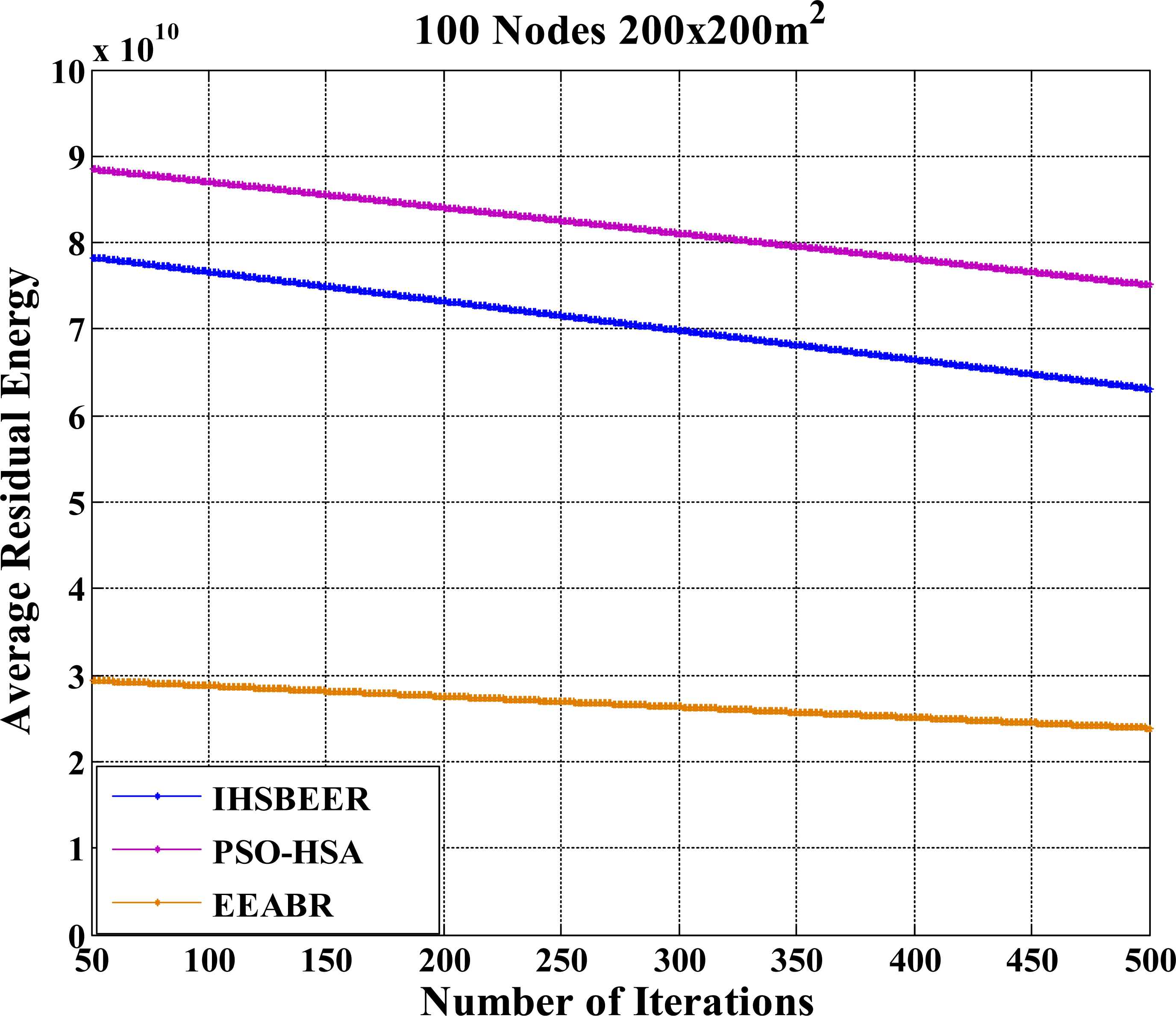
Average Residual Energy EEABR, IHSBEER and PSO-HSA (10 clusters)
Average Residual Energy EEABR,IHSBEER and PSO-HSA(10 clusters)
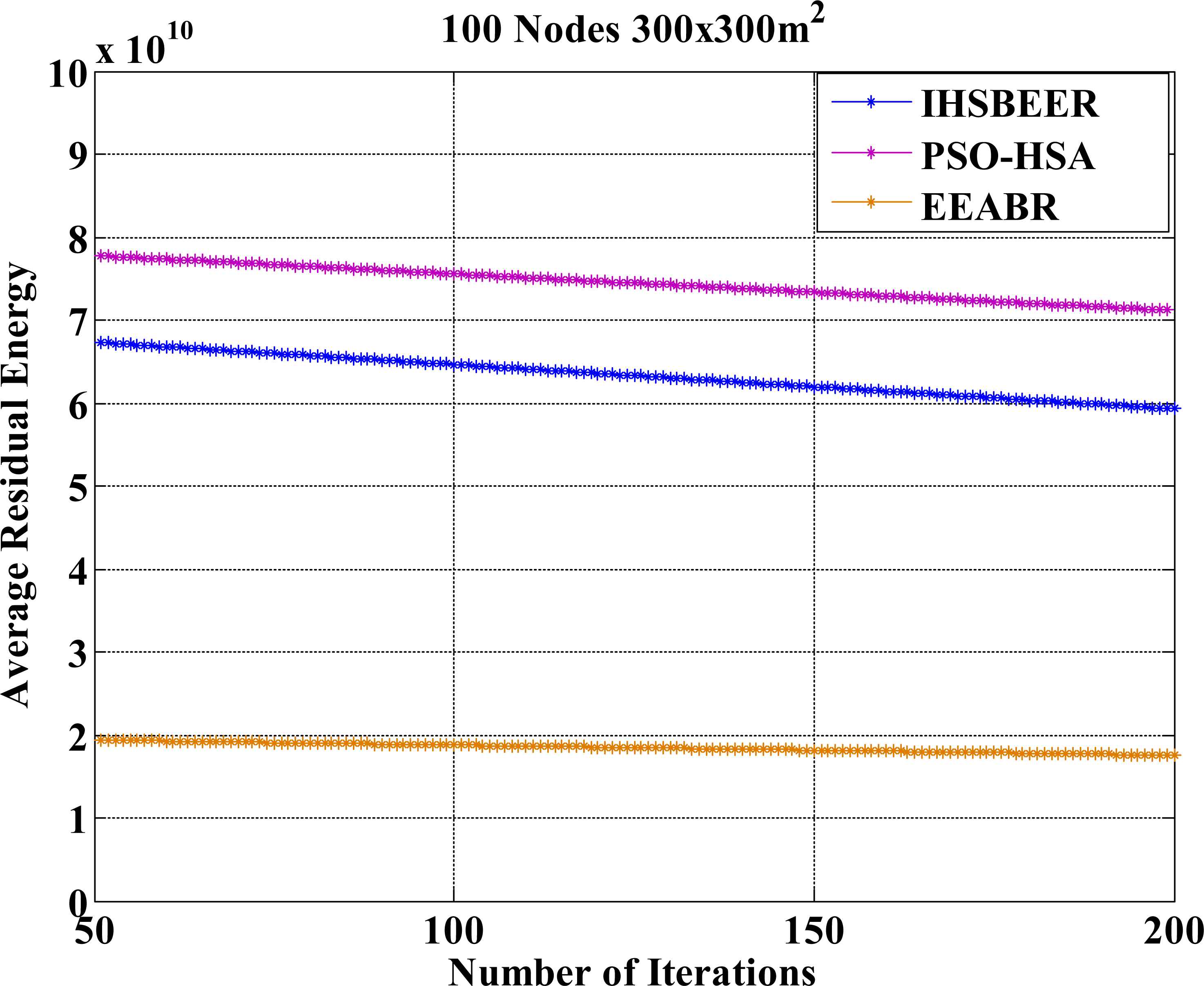
When path is created, it is easy to forward data through that path. But when any node in the path get exhausted (becomes less than threshold energy) that node will be removed from the path and new path will be generated. They remove the traffic load and allow their preceding GN node to communicate directly to the BS. Thus, the energy consumption due to these GN decreases due to transmission of large amount of traffic load to nearby GN. Fig 4 shows the result for 100 node in 300×300 m2 area with 10 clusters. Fig 5 shows the result for 100 node in 400×400 m2 area with 10 clusters.
Average Residual Energy EEABR,IHSBEER and PSO-HSA(10 clusters)
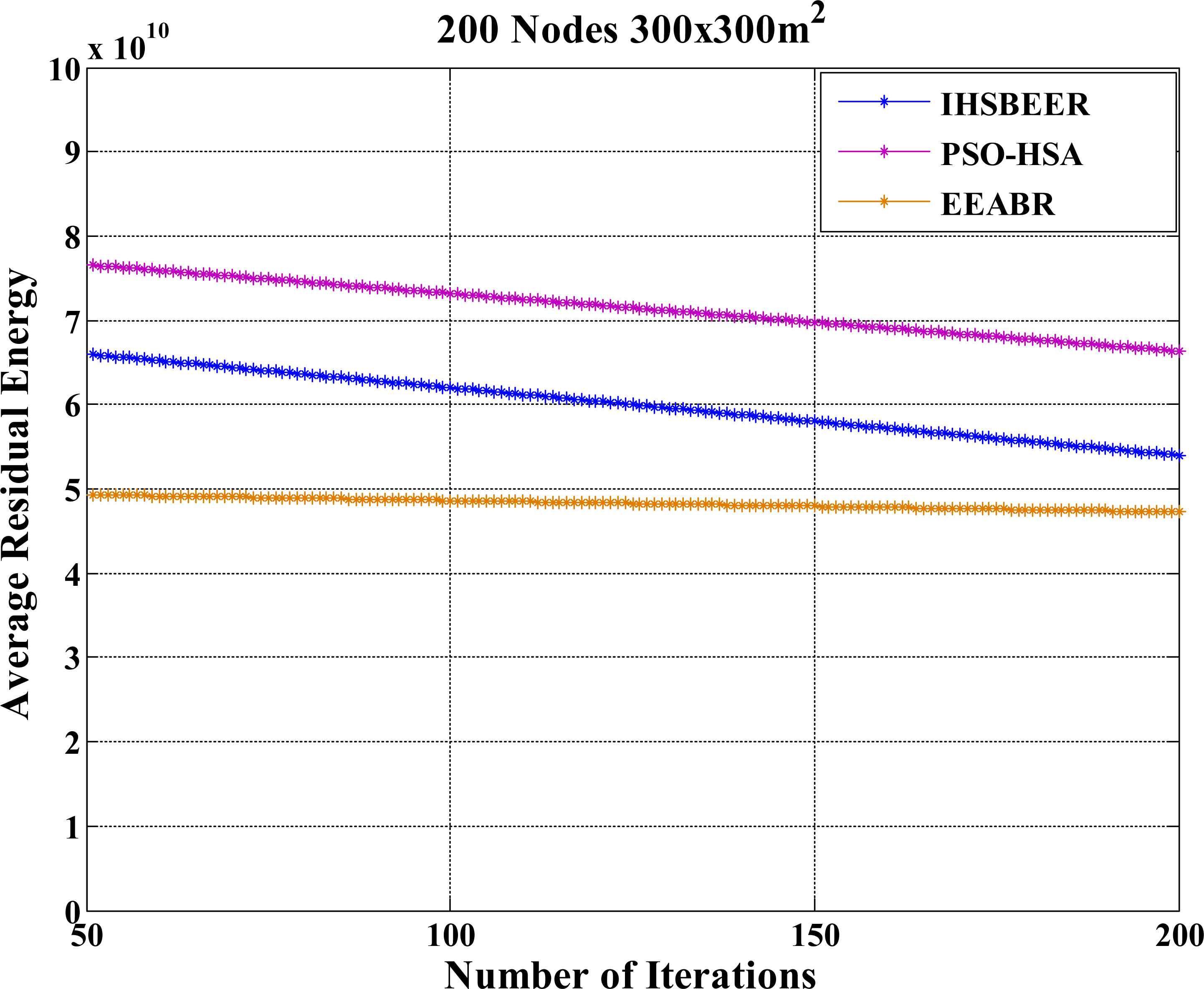
Fig 6 shows the result for 200 node in 300×300 m2 area with 20 clusters. Fig 3–8 represents Average residual energy for varying number of nodes, network area and number of clusters. Here 10% of clusters are taken for each network scenarios. The main cause of energy maximization is introduction gateway nodes and data forwarded by best routing path to the sink. As a result, the proposed algorithm showing better results. Also, the average residual energy is higher because it distributes the traffic over the cluster head and gateway node in order to balance the transmission cost.
Average Residual Energy EEABR,IHSBEER and PSO-HSA(20 clusters)
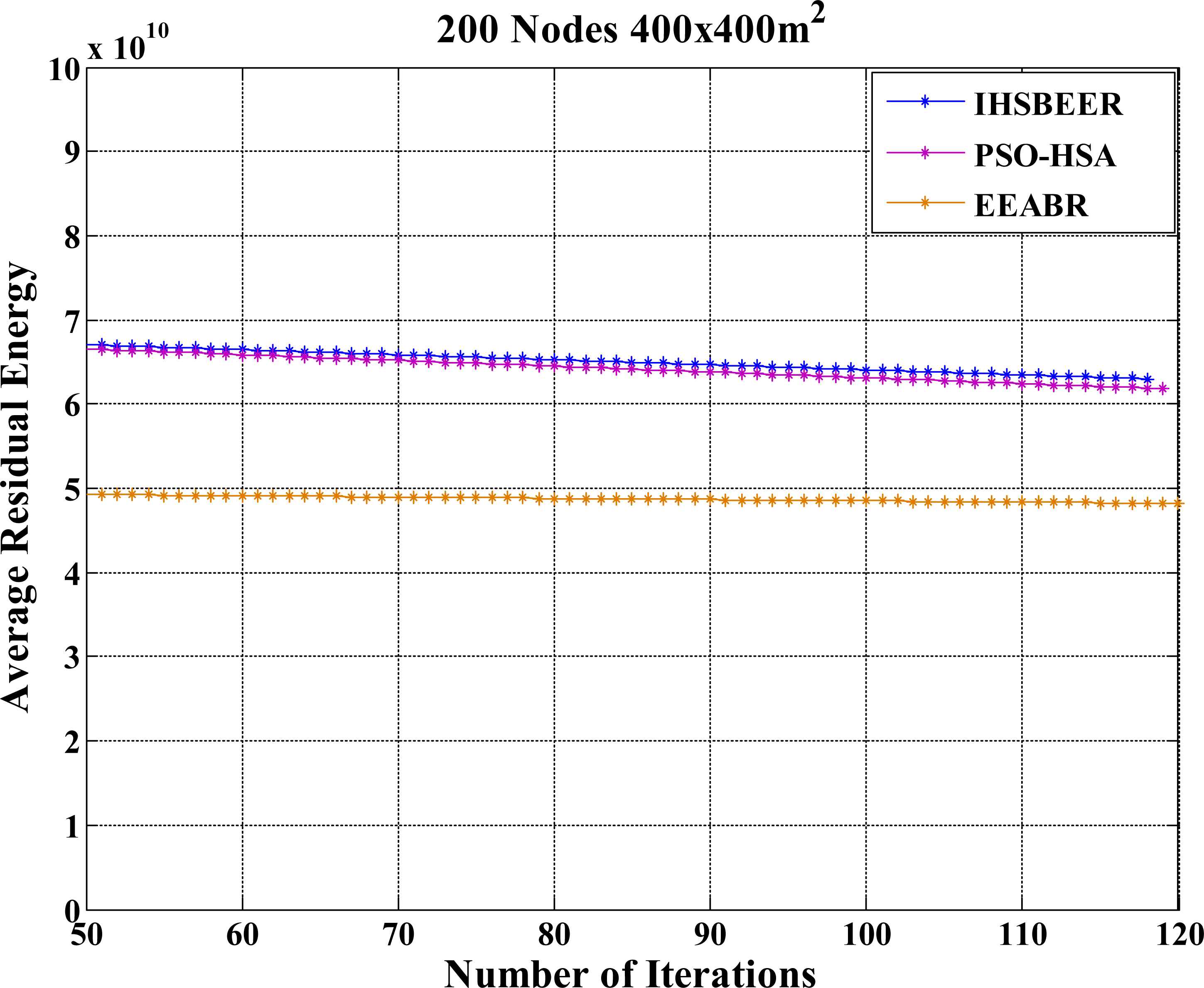
The above Fig 3–8 shows the average residual energy by the simulations done by EEABR and the IHSBEER algorithms. The iterations continue until one of the nodes reaches a specified threshold value, (taken here as 40% of the total energy stored by the node) after which it is considered as dead node and the data transmission through that path stops. Fig 7 shows the result for 200 node in 400 × 400 area with 20 clusters. Fig 8 shows the result for 300 node in 200×200 area with 30 clusters. This shows that the PSO-HAS algorithm is consuming energy at a slower rate than other algorithms.
Average Residual Energy EEABR,IHSBEER and PSO-HSA(20 clusters)
Average Residual Energy EEABR,IHSBEER and PSO-HSA(20 clusters)
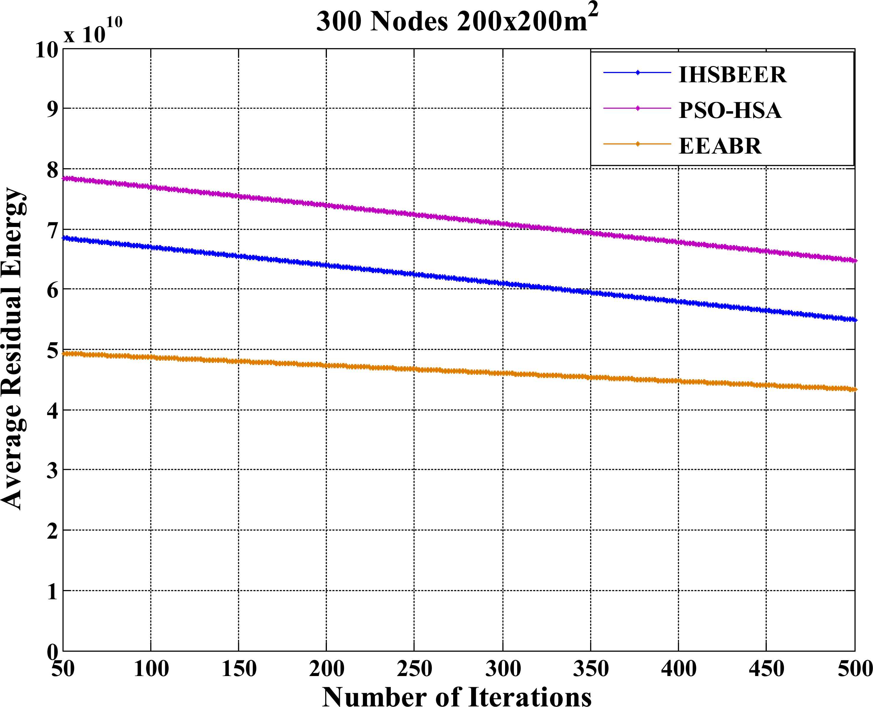
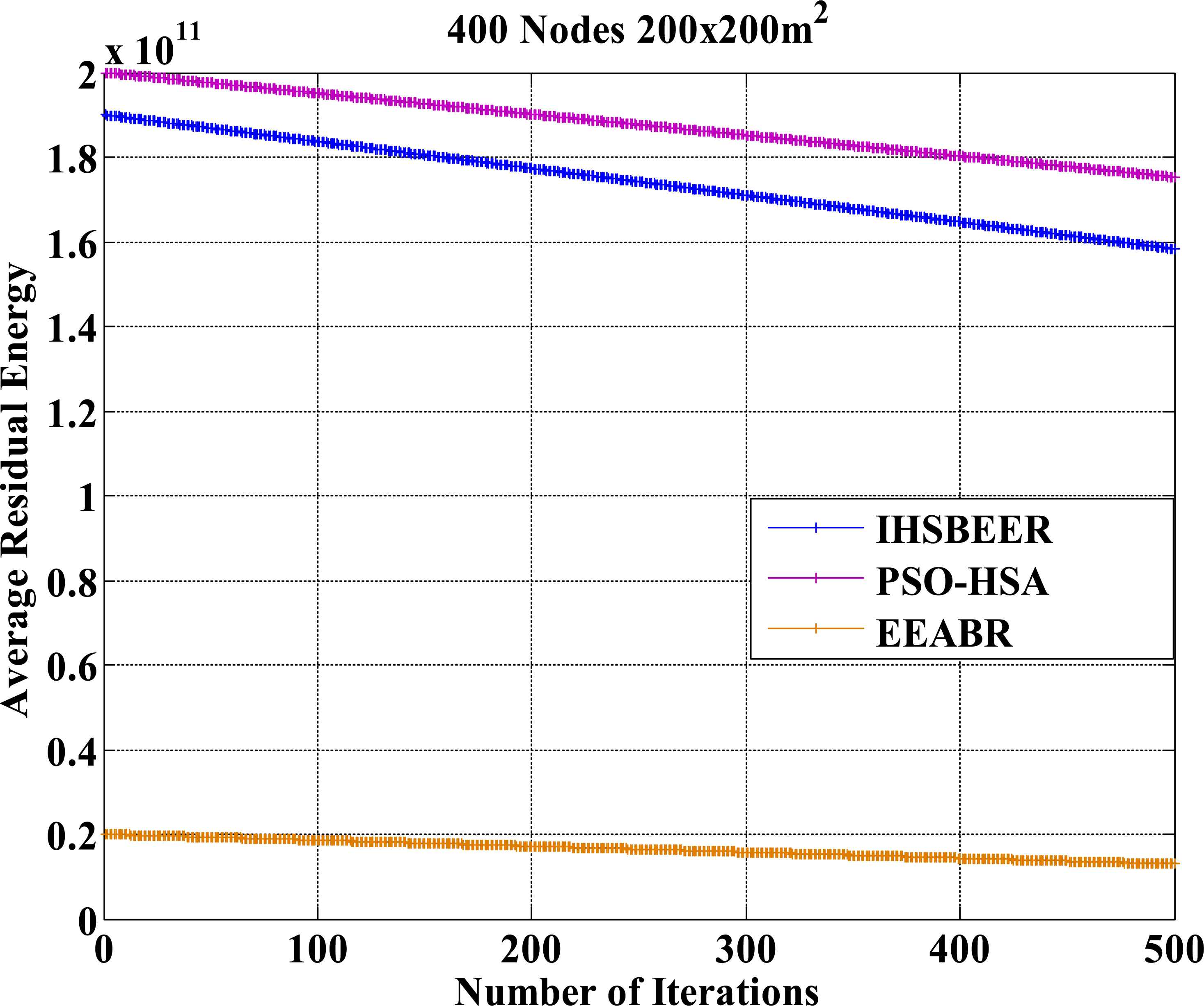
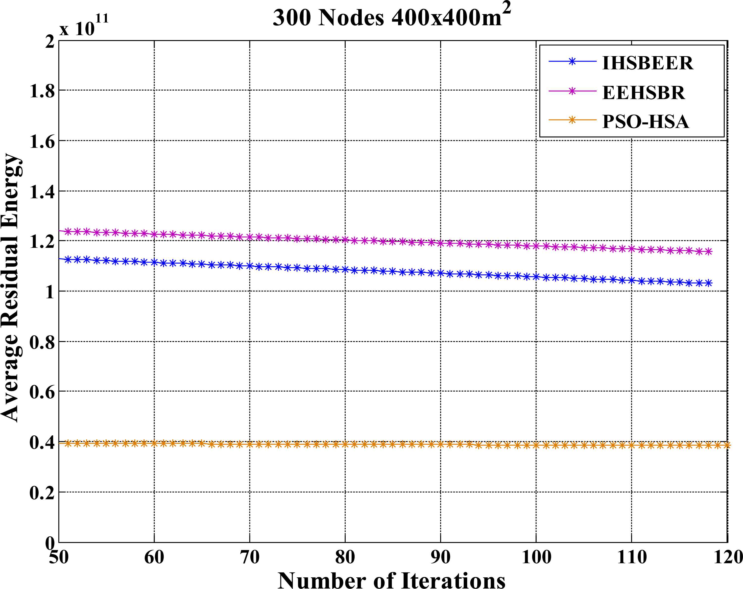
Fig 9 shows the result for 300 node in 300×300 m2 area with 30 clusters. Fig 10 shows the result for 300 node in 400×400 m2 area with 30 clusters. Fig 11 shows the result for 400 nodes in 200×200 m2 area with 40 clusters. Fig 12 shows the result for 400 node in 300×300 m2 area with 40 clusters. Initially up to certain rounds, average residual energy is much higher for the proposed algorithm than that of other existing algorithms. This is also depicted in Fig. 9–12 in terms of energy remaining for 300-400 sensors nodes, which is much higher than the existing algorithms.
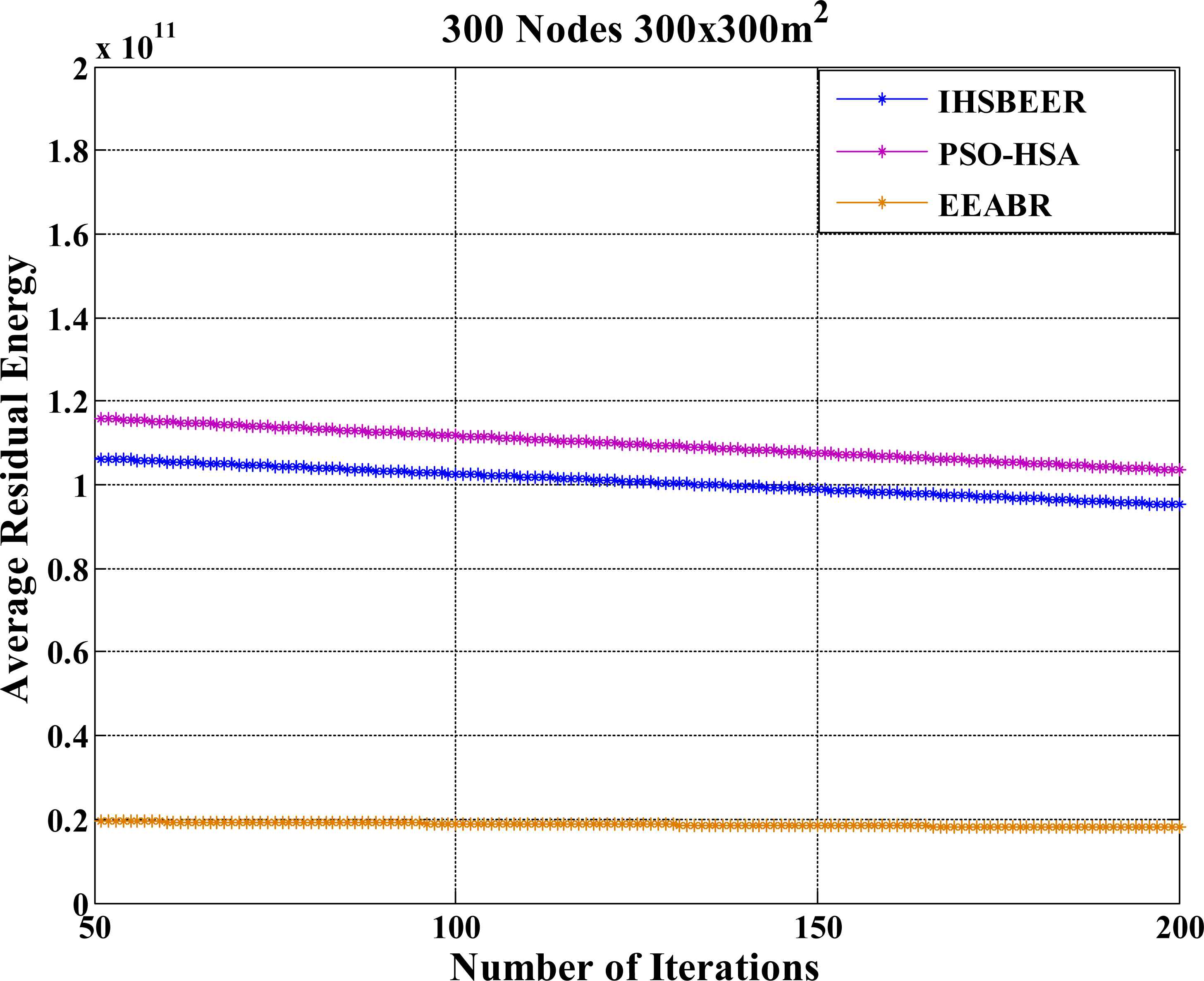
Average Residual Energy EEABR,IHSBEER and PSO-HSA(30 clusters)
Average Residual Energy EEABR,IHSBEER and PSO-HSA(30 clusters)
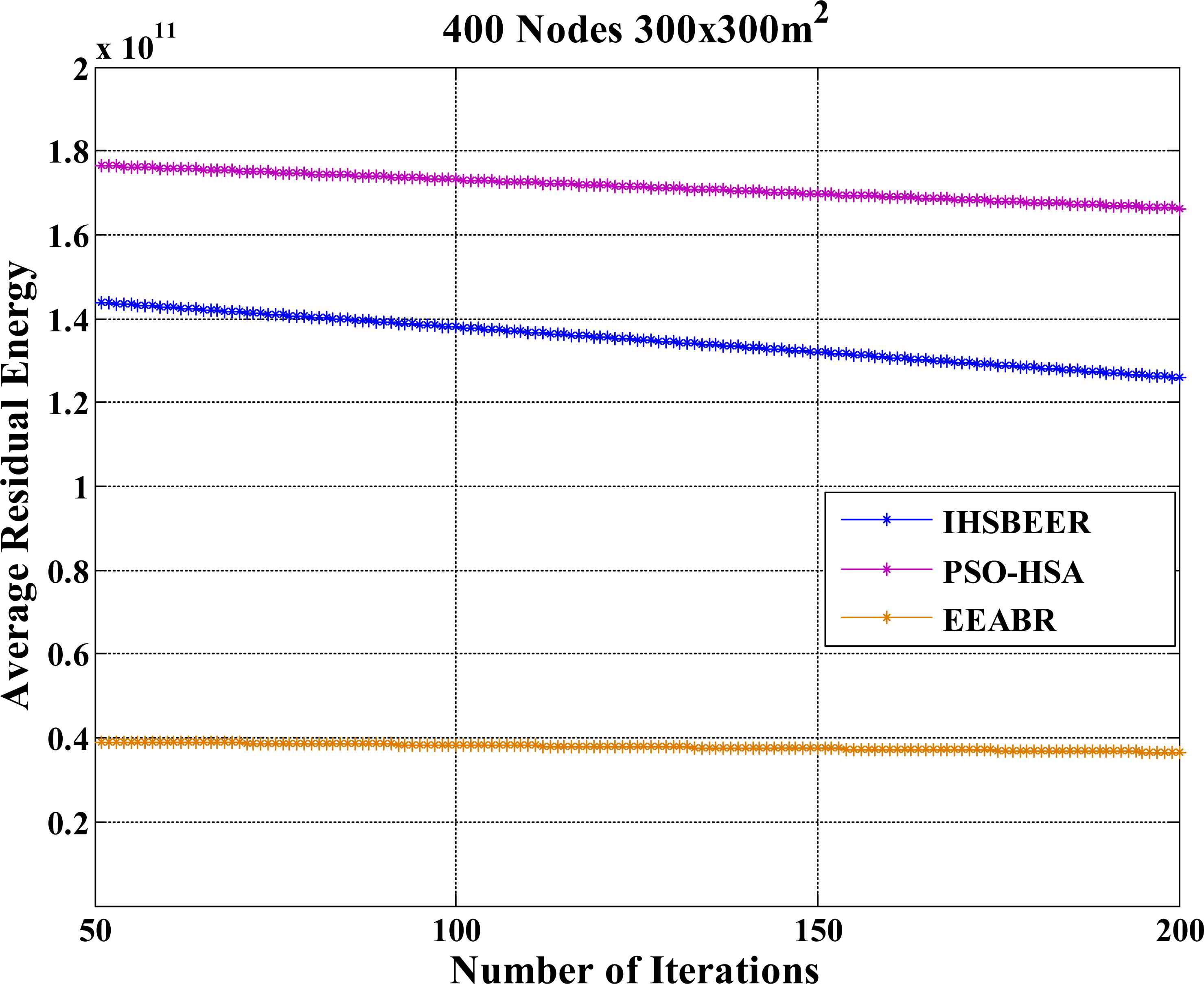
Average Residual Energy EEABR,IHSBEER and PSO-HSA(40 clusters)
Average Residual Energy EEABR,IHSBEER and PSO-HSA(40 clusters)
The residual energy of the network in the proposed approach is much higher than the others, because it distributes the traffic load over the CHs and gateway nodes.
5. Conclusion
In this paper, PSO-HSA based algorithm, where PSO is used for cluster head selection is optimized, and HSA based routing used for the selection of best route. The proposed approach is efficient as it include selection of optimal cluster through fitness function and route selection using HSA. The introduction of Gateway node using PSO reduces the distance between the cluster head and sink and best routing path is established using harmony search to eases the further communication between them. The simulation results show that PSO-HSA algorithm performs better than other conventional protocols such as EEABR and the IHSBEER and can extend the lifetime of the network.
References
Cite this article
TY  - JOUR
AU  - Veena Anand
AU  - Sudhakar Pandey
PY  - 2017
DA  - 2017/07/24
TI  - Particle Swarm Optimization and harmony search based clustering and routing in Wireless Sensor Networks
JO  - International Journal of Computational Intelligence Systems
SP  - 1252
EP  - 1262
VL  - 10
IS  - 1
SN  - 1875-6883
UR  - https://doi.org/10.2991/ijcis.10.1.84
DO  - 10.2991/ijcis.10.1.84
ID  - Anand2017
ER  -