
Generalized fuzzy trees
- DOI
- 10.2991/ijcis.2017.10.1.47How to use a DOI?
- Keywords
- Generalized fuzzy graphs; trees; effective edges; strongly connected graphs; bridge
- Abstract
Graphs are the backbone of many real systems like social networks, image segmentation, scheduling, etc. To input uncertainty to such systems, generalized fuzzy graphs are used. Generalized fuzzy tree is one generalized fuzzy subgraph of a generalized fuzzy graph which characterizes the whole graph. In this study, generalized fuzzy trees are introduced. The concepts of strongly connectedness, nearly disconnect, distance between two nodes, bridges are exemplified.
- Copyright
- © 2017, the Authors. Published by Atlantis Press.
- Open Access
- This is an open access article under the CC BY-NC license (http://creativecommons.org/licences/by-nc/4.0/).
1. Introduction
Motivation of graph theory is present from Leonhard Euler(1730) paper of the problem for seven bridges of köningsberg. Graphs are very important tools for expressing the relationships among units, which are represented by nodes. Relationships among nodes are expressed by connections. In general, any system involving points and lines among them can be represented as a graph. At present, graph theory is a large field of research for theory and applications both. For, further of graph theory, readers may look into 6.
Nowadays, graphs do not represent any systems properly due to the uncertainty or haziness of the parameters of systems. For example, a social network may be expressed as a graph where nodes express an account (person, institution, etc.) and edges represent the relation between the accounts. If the relations among accounts are measured as good or bad according to the frequency of contacts among the accounts, fuzzyness can be added for such representation. This and many other problems lead to define fuzzy graphs. The first concept of a fuzzy graph was established by Kaufmann 8 in 1973. But, it was Rosenfeld25 who discussed relations on fuzzy sets and improved the theory of fuzzy graphs in 1975. Using this concept of fuzzy graph, Koczy 10 used fuzzy graphs in the optimization of networks. For further details of fuzzy graphs, readers may look in 7,9,11,12,15,16,17,18,19,20,21,22,23,27.
There are several types of fuzzy graphs available in the literature. Intuitionistic fuzzy graph 14, interval-valued fuzzy graphs 1, and bipolar fuzzy graphs 2 are some of them. In all these fuzzy graphs, there is a common property that edge membership value is less than to the minimum of it’s end node membership values. Suppose, a social network is to be represented as fuzzy graphs. Here, all social units are taken as fuzzy nodes. The membership values of the nodes may depend on several parameters. Suppose, the membership values are measured according to the sources of knowledge. The relation between the units is represented by fuzzy edge. The membership value is measured according to the transfer of knowledge. But, transfer of knowledge may be greater than one of the social actors/units as more knowledgeable person informs less knowledgeable person. But, this concept can not be represented in fuzzy graphs as edge membership value should be less than membership values of the end nodes. Thus, all images/networks can not be represented by fuzzy graphs. To remove the restriction, generalized fuzzy graphs are introduced.
In 1999, Sunitha 24 et al characterized the fuzzy trees. They have used the concept of strong edges. This concept depends on all edges of a graph. But, it is comparative and hard to compute for an edge to be strong or not. In this paper, effective edges are defined. Effective edges are easy to compute and non-comparative. According to the effectiveness, trees are defined here. For further details of tree, readers may look into 13,26. Akram et al. 3,4,5 defined different types of trees namely soft trees, fuzzy soft tress and bipolar soft trees.
After introductory section, some basic notions are discussed in Section 3. In that section, Generalized fuzzy graphs of type 1 and type 2 (GFG1, GFG2) [Section 3.1] are described with suitable examples. In Section 3.2, generalized fuzzy directed graphs are described. In Section 4, generalized fuzzy trees are introduced. After that, in Section 5, distance function and distance between two nodes are discussed. In Section 6, strongly connected GFGs are described with suitable examples. Here, bridges are also defined. In Section 7, generalized fuzzy directed trees are introduced and some properties are proved. Insights of this study are discussed in the Section 8. At last, conclusion is drawn in Section 9.
2. Problem definition of this work
This study focuses on generalization of fuzzy trees (GFTs) and generalized fuzzy directed trees (GFDTs). In this paper, it is considered that any generalized fuzzy graph (GFG) which is a cycle in crisp sense may be considered as a tree if it fulfills the criteria of trees. Length between two nodes in GFT is to be measured. Also, Strongly connected GFTs will be discussed. Also, the sufficient rule for a cycle to be a GFT will be established.
3. Preliminaries
A fuzzy graph ξ =(U, σ, μ) is a non-void set V with a pair of mappings σ : V → [0, 1] and μ: U × U → [0, 1] as if for each x, y ∈ V, μ(x, y) ⩽ σ(x) ∧ σ(y).
Underline crisp graph of a fuzzy graph ξ = (U, σ, μ) is |ξ| =(U, E) with E = {(x, y)|μ(x, y) ⩾ 0}.
3.1. Generalized fuzzy graphs (GFGs)
The membership value of nodes of graphs depend on membership values of the adjacent edges. For isolated nodes, the membership values of nodes are taken as 0. The membership mapping is defined from a non-void set to a closed interval [0,1]. Thus, any linguistic term can be defined by membership values. Some times, node membership values are considered first and depending on node membership values, the edge membership values can be considered. For example, social networks, where social actors and its stability are considered first. Depending on stability, node membership values are given. After that, relation among the actors are considered. The membership values may be taken from the parameter ‘relationship’. Again, in some problems, edges are considered first and depending on edge membership values the node membership values are considered. For example, capacities of pipelines can be taken as edge membership values and depending on the capacities, node membership values are decided.
Thus, two types of relations are assumed. In the following, generalized fuzzy graphs of first kind is defined. Here, node membership values are considered first. Then, depending on node membership values, edge membership values are considered.
| Authors | Year | Contributions |
|---|---|---|
| A. Kauffman8 | 1973 | Introduction of fuzzy graphs. |
| A. Rosenfeld25 | 1975 | Modification of the concept of fuzzy graphs given by Kauffmen 8. He added that edge membership value is less than minimum of node membership values. |
| M. S. Sunitha et al24 | 1999 | Characterization of fuzzy trees. |
| J.Yun et al26 | 2014 | Fuzzy decision trees. |
| M. Akram et al5 | 2016 | Fuzzy soft trees. |
| S. Samanta et al21 | 2016 | Introduction of generalized fuzzy graphs. |
| This paper | – | Characterisation of generalized fuzzy trees and its properties. |
Authors’ contributions towards generalized fuzzy trees.
Definition 1.
21 Let V be a non-void set. Two mappings are considered as follows: ρ: V → [0, 1] as well as ω: V × V → [0, 1], A = {(ρ(x), ρ(y))|ω(x, y) > 0}. The triad (V, ρ, ω) is said to be generalized fuzzy graph of first kind (GFG1) if there exists a mapping ϕ: A → (0, 1] such that ω(x, y) is equal to ϕ((ρ(x), ρ(y))), where x, y ∈ V.
Now, generalized fuzzy graphs of second kind is defined. Here, the membership values of edges are considered first. Then, depending on edge membership values, node membership values of nodes are assigned.
Definition 2.
21 Let V be a non-void set. Two mappings are considered as follows: ρ: V → [0, 1] and ω: V × V → [0, 1]. Also, let B be the range set of ω. The triad (V, ρ, ω) is said to be generalized fuzzy graph of second kind (GFG2) if there exists a mapping ψ: B → (0, 1] with the rule that for each x ∈ V, ρ(x) is equal to ψ(ω(ex)) where ex = (x, y) such that y ∈ V.
Note 1 In GFG2, the co-domain set of ψ excludes the number 0, as the membership values of nodes are always positive.
The order of GFG, ξ is O(ξ) = ∑x∈Vρ(x). The size of GFG, ξ is S(ξ) = ∑x, y∈Vω(x, y).
3.2. Generalized fuzzy directed graphs (GFDGs)
The generalized directed fuzzy graph of first kind (GDFG1) is defined below.
Definition 3.
Let V be a non-void set. Two mappings are considered as follows: ρ: V → [0, 1] as well as
Example 1.
Let the node set be V = {x, y, z, t} and edge set be
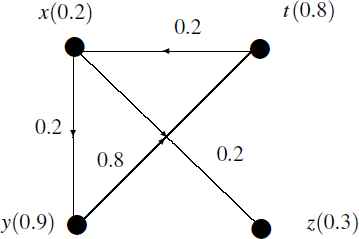
A generalized directed fuzzy graph of first kind (GDFG1)
Degree of a node x in GDFG1 is the pair (d+(x), d−(x)) where d+(x), out degree of x, is the sum of the generalized membership values of outgoing edges and d–, in degree of x, is the sum of the generalized membership values of incoming edges. Thus,
Note 2 In GDFG1, out degree or in degree of a node may be 0. But, when both are 0 then the node is called null node.
Generalized directed fuzzy graph of second kind (GDFG2) is introduced below.
Definition 4.
Let V be a non-void set. Two mappings are considered as follows: ρ: V → [0, 1] and
By the Definition, 4 it is true that, if a node has no incoming edge but has outgoing edges, its generalized membership value is 0. Let us discuss this situation with an example.
Example 2.
Now, it is true that V = {a, b, c, d, e}. The edge membership values are given as
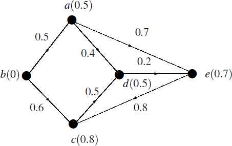
A generalized directed fuzzy graph of second kind (GDFG2)
Degree of a node x in GDFG2 (similarly defined) is the pair (d+(x), d−(x)), where d+(x), out degree of x, is the sum of the generalized membership values of outgoing edges and d−, in degree of x, is the sum of the generalized membership values of incoming edges. Thus,
Note 3 In GDFG2, in-degree and (or) out-degree of a node may have chance to be zero. If they are zero, the node is said to null node.
4. Generalized fuzzy trees
In general, if the membership value of an edge is greater than half of its maximum of membership values of its end nodes, the edge is said to be an effective edge. Suppose, someone informs another person about any news. If the transfer of knowledge is greater than to a minimum amount (may be assumed half of the source knowledge), then the second person can be informed effectively. Thus, transfer of knowledge (which indicates the membership value of an edge) helps a person (a node with lower membership value) to get more knowledge from a source (a node with greater membership value). Formal definition of an effective edge is given below.
Definition 5.
Let ξ = (V, ρ, ω) be a GFG1 (or GFG2). An edge (x, y) is said to be effective edge if
Note 4 It is obvious that for GFG1, ω(x, y) = ϕ(x, y). Now, if an edge of a generalized fuzzy graph is effective, then other edges may not be effective. The following is the analytic description of this statement. Let ξ be a GFG1 and it has the node set {a(0.8), b(0.2), c(0.3)} and the edge set {(a, b), (b, c)} and ϕ(x, y) = min{x, y}. Then ϕ(a, b) = 0.2, ϕ(b, c)= 0.2. The edge (b, c) is effective as
A GFG ξ′ =(V′, ρ′, ω′) is a subgraph of ξ = (V, ρ, ω), if V′ ⊂ V, ρ′: V′ → [0, 1] as well as ω′: E′→ [0,1], where E′ ⊂ V′ × V′ such that ρ′ (x) ⩽ ρ(x) as well as ω′ (x, y) ⩽ ω(x, y). Spanning subgraphs contain all nodes of the graph. If all the edges of the spanning subgraph are effective, then the sub-graph is called effective spanning subgraph. Now, the definition of generalized fuzzy trees (GFTs) is introduced below. In this study, if a GFG is mentioned, it is connected in crisp sense, i.e. all nodes are connected by a path whether the edges of the path may be effective or not.
Definition 6.
A GFG ξ = (V, ρ, ω) is a generalized fuzzy tree (GFT) if it has an effective spanning subgraph ℱ =(V, ρ′, ω′) whose underline crisp graph is a tree and all arcs (u, v) not in ℱ are not effective.
Example 3.
In Fig. 3, a GFT is shown. The normal lines are effective and dotted lines are non-effective. Thus, the graph contains a subgraph whose all edges are effective. It is easy to observe that the underline graph is a tree. Hence, the graph of Fig. 3 is a GFT.
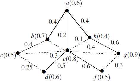
A GFT (dotted lines are not effective).
In classical theory of graphs, crisp trees with n nodes have n − 1 edges. But, GFT of n nodes may contain more than n − 1 edges. The graph may contain a cycle in crisp sense. The following statement describes the consequence of the theorem of classical theory.
Note 5 A GFT of n nodes contains n − 1 effective edges.
The reverse of the statement is not true. A graph may have n − 1 effective edges but still not GFT. For example, in Fig. 4, there are 3 effective edges of a GFG with 4 nodes. As an effective spanning sub-graph is not found in the graph, the graph can not be a GFT.
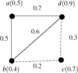
A GFG with 4 nodes and 3-effective edges but not GFT
If underline graph of a GFG is a crisp cycle, then the GFG is called a cycle. Every such cycle may be a GFT. This statement can be established from the following theorem.
Theorem 1.
Every cycle is a GFT if and only if the cycle has only one non-effective edge.
Proof
Let ξ =(V, ρ, ω) be a cycle. Also let, ξ be a GFT. Then there exists an effective spanning tree. As spanning tree contains all the nodes of ξ, one edge must be removed from cycle to construct spanning tree. Hence, that edge must be non-effective. The conclusion is that every cycle which is a GFT must contain a non-effective edge.
Conversely, let ξ =(V, ρ, ω) be a cycle and it has only one non-effective edge. If the non-effective edge is removed from the cycle, it becomes a tree in crisp sense. Also, all the edges of the spanning subgraph are effective and it includes all the nodes of the graph. Hence, ξ is a GFT.
Theorem 2.
Let ξ be a GFG of n nodes and its underline crisp graph be complete. If ξ is GFT, then it has
Proof
In complete graph of n nodes, the edge number is
Note 6 The converse of the statement is not correct. Suppose a GFG has 4 nodes, then it may have maximum 6 edges. If it has
5. Length between two nodes in GFT
The definition of distance mapping is given below.
Definition 7.
Let us consider ξ = (V, ρ, ω) be a GFG. Now, the length mapping on ξ is dξ : E → R, where E is the edge set of ξ with the following rule:
For each x, y ∈ V
- (i)
dξ(x, y) is greater or equal to 0
- (ii)
dξ(x, y) is equal to dξ(y, x).
Paths are very important and useful concept in graphs. One node may not be connected directly. By different paths, many nodes may be connected. In fuzzy graphs, paths are of different types. A path is said to be strong if all edges of the path are effective. Otherwise, i.e. at least one edge is not effective, the path is called weak path. Now, the lengths between two nodes are stated as follows:
Definition 8.
Let ξ = (V, ρ, ω) be a GFG with the length mapping on ξ as dξ: E → R, where E is the edge set of ξ. The length measurement within the nodes x as well as y is D(x, y) = min(P∈𝒫) (dξ(x, u1) + dξ(u1, u2)+ ... + dξ(uk, y)), where ui ∈ P, i = 1, 2,..., k as well as 𝒫 is a set of every paths between x and y.
In this paper, the length is measured according to the effectiveness of the edges. The effectiveness of an edge (x, y) in GFG is determined as
Example 4.
In Fig. 4, the length between the nodes b and d is to be measured. Here, the number of paths between b and d are P1: {b → a → d}, P2: {b → d} and P3: {b → c → d}. Now, the length between the nodes along the path P1 is
Note 7 Triangle inequality does not hold for fuzzy length.
This statement is verified in the Example 4. Here, D(b, d) = 0.62, D(b, c) = 0.285, D(c, d) = 0.333. Thus, D(b, d) = D(b, c) + D(c, d).
The centre of a GFG is defined below. Let ξ = (V, ρ, ω) be a GFG. The centre of the GFG is the set of nodes whose lengths from farthest nodes are minimum. Now for large networks, it is convenient that the nodes with approximately same lengths from farthest nodes are to be considered. Before the formal definition of centre, definition of farthest nodes from a node are defined here.
Definition 9.
Let ξ = (V, ρ, ω) be a GFG. The farthest nodes of x is the set of nodes Fx = {z|D(x, z) > D(x, y)∀y ∈ V}.
Generalization of the definition of centre is given below.
Definition 10.
Let ξ = (V, ρ, ω) be a GFG. Also, let ε > 0 be a small pre assigned positive number such that 0 ⩽ ε ⩽ 1. The centre of ξ is the set C = {x|D(x, y) + ε < D(t, z)∀t ∈ V|y ∈ Fx, z ∈ Ft}
Example 5.
In Fig. 4, the farthest node of a is c with the length 1.21, that of b is a with the length 1. Similarly, for other nodes c and d, the farthest nodes are a (with length 1.21) and a (with length 0.77). So the node with minimum lengths from their farthest node is d. Hence, the centre of the graph is d. Now, if generalization concept is used, and take ε = 0.3, then the centre of the graph is C = {d, b}.
Radius and diameter are also defined. Radius is the length from the center(s) to the farthest node in a GFG. On the other hand, diameter is the length measurement between two end nodes of a longest path (a path with maximum length).
6. Strongly connected GFG and spanning GFT
In this paper, it is assumed that a tree may contain effective and non-effective edges. It is known that a spanning tree includes all nodes of the graph.
Definition 11.
Let T = (V, ρ, ω) be a GFT. T is defined to be spanning tree of a GFG, ξ if T is a subgraph of ξ and T contains all nodes of ξ.
Thus, every GFG may or may not contain spanning tree. Here, connectivity of a graph is represented in terms of spanning tree. The following study introduces two concepts namely, strongly connected and nearly disconnected GFG.
Let ξ = (V, ρ, ω) be a GFG. If the GFG has a spanning tree, then it is strongly connected (Type 1). If GFG does not contain any spanning tree, then the graph may contain one or more trees as sub-graphs. In that case, two cases may arise. Some nodes are not incident to effective edges. Suppose, every such node, say x, is connected by some non-effective edges, say (x, y1), (x, y2), ..., (x, ym) with the rule
Example 6.
In Fig. 5(a), a GFG is drawn. The dotted lines are non-effective and normal lines are effective. In the figure, a spanning tree is shown. Thus, the graph is strongly connected GFG of type 1. In Fig. 5(b), a node x is incident to non-effective edges (x, y1), (x, y2), (x, y3), (x, y4). If it is assumed that
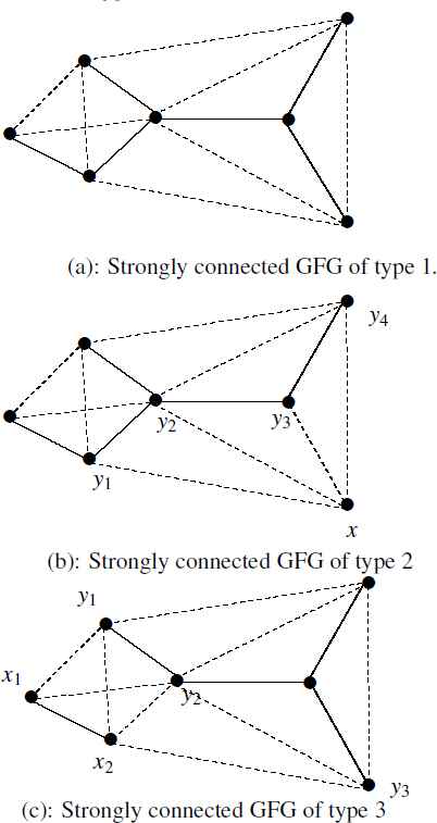
Strongly connected GFGs
On the other hand, weakly connected graphs are the graphs which are not strongly connected. Now, nearly disconnected graphs are defined below. Let ξ = (V, ρ, ω) be a GFG. Let ε be a small positive number such that 0 < ε < 0.5. If the graph contains a spanning GFT, then the graph is strongly connected. If a graph does not contain an effective spanning tree, there may arise two cases. Firstly, some nodes are not incident to effective edges. Suppose, every such node, say x, is connected by some non-effective edges, say (x, y1), (x, y2), …, (x, ym) such that
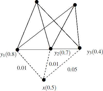
Example 7.
Let us consider a GFG shown in Fig. 6 and ε = 0.13. Here, a node x is connected to nodes y1, y2, y3. Also, sum of the effectiveness of the edges (x, y1), (x, y2), (x, y3) is 0.1268 < ε. As the graph contains at least one such node with weak effectiveness, then the graph is nearly disconnected.
Theorem 3.
Let ξ be a GFG whose underline graph is a cycle. Also let, ξ has no effective edges. Then ξ is strongly connected if sum of effectiveness of any pair of edges of ξ is greater than 0.5.
Proof
Here, ξ is a GFG whose underline graph is a cycle. Also, ξ has no effective edges. Let x be any node of ξ with the rule (x, y) and (x, z) are incident edges. Now, according to the rule,
An example of nearly disconnected graph
In the theory of graphs, bridges are such edges whose removal disconnects the graphs. Now, bridge in GFG is introduced as follows:
Definition 12.
An edge in strongly connected GFG is said to be bridge if its removal turns the graph as nearly disconnected.
In the Definition 7, it is easy to verify that bridge is an effective edge (type 1) or non-effective edges (type 2). The following example verifies the definition properly.
Example 8.
Let us assume that ε = 0.25. In the Fig. 7, normal lines are effective edges and dotted lines are non-effective edges. Now, it is easily seen that the edge (y, z) is a bridge if effectiveness of (x, y) is less than 0.25.
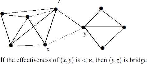
A bridge in GFG
It is easy to state that a GFT whose underline graph is cycle, has only one non-effective edge. If another edge is non-effective, then the graph has the following property.
Theorem 4.
Let ε be a small pre assigned positive number such that 0 < ε ⩽ 0.5. Every edge in a GFT whose underline graph is cycle, is a bridge if the effectiveness of the non-effective edge of the GFT is less than ε.
Proof
Let ε be a pre assigned small positive number such that 0 < ε ≤ 0.5. Let ξ be a GFT whose underline graph is a cycle. It is easy to state that a GFT whose underline graph is cycle, has only one non-effective edge. By the definition of bridge, an edge is said to be bridge if its removal, creates the graph as nearly disconnected. Thus, if every edge is a bridge in ξ, then effectiveness of the non-effective edge is less than ε.
7. Generalized fuzzy directed trees
The definition of generalized fuzzy directed trees (GFDTs) can be similarly introduced. A GFDG is said to be GFDT, if it has effective spanning directed tree.
Definition 13.
A GFDG ξ =(V, ρ, ω) is a generalized fuzzy directed tree (GFDT) if
- (i)
it has an effective spanning subgraph ℱ = (V, ρ′,ω′) whose underline crisp graph is a tree and all arcs (u, v) not in ℱ are not effective.
- (ii)
one node, say a, of ℱ has null in-degree, i.e. d−(a) = 0.
A GFDT is shown in Fig. 8. Here, dotted lines are non-effective edges. Thus, in GFDT, there is no cycle whose all edges are effective.
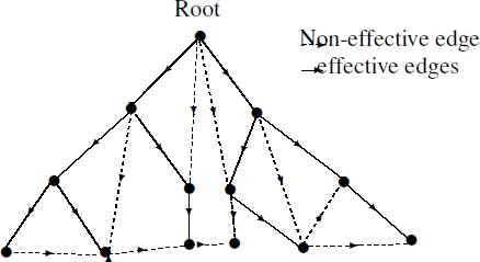
Generalized directed fuzzy trees
In GFDT, there is one node whose in-degree is less than all other nodes. In GFDT, there is a node in which all effective edges are out-coming and incoming edges are non-effective, if there be any. This special node is known as root of GFDT. The information regarding the in-degree nodes in GFDT, can be found in the following theorem.
Theorem 5.
Let ξ be a GFDT. The effectiveness of each in-coming edges is greater than 0.5 except root.
Proof
Let ξ be a GFDT. Now, ξ has a spanning tree. By the definition of spanning tree, all edges of the tree are effective. Hence, all nodes in the tree has in-coming effective edges exactly once. Thus, the effectiveness of the in-coming edges are greater than 0.5. The only node, the root has no effective in-coming edge.
8. Insights for this study
- •
GFTs are introduced. Cycles in crisp sense are not assumed as trees, but in this case if the cycle has one weak edge, it may be assumed as trees.
- •
Length within nodes in GFT is introduced. Depending on the definition, centre and radius are described.
- •
Strongly connected trees and spanning trees are discussed. Thus, a cycle may be assumed as spanning tree but strongly connected cycle is not considered as spanning trees. This is the importance of strongly connected graphs.
- •
The rule of a cycle to be tree is established. The rule of a GFG to be nearly disconnected is also provided.
- •
Generalized fuzzy bridge is described. Also, GFDTs are defined and some properties are given.
9. Conclusions
This study described a major part of generalized fuzzy graphs known as generalized fuzzy trees. Length between two nodes were assumed as effectiveness of the corresponding edges. Also, the length may be measured by some other ways depending the application and expert opinion. Strongly connected and nearly disconnected graphs were discussed. For nearly disconnected GFG, it was assumed that ε satisfies the inequality 0 < ε ⩽ 0.5. This assumption could be changed as per application. According to different situations ε can be changed. Also, bridges in GFG were discussed. For an image representation, objects were assumed as effective edges, and backgrounds were taken as the non-effective edges in GFGs. In Wassenberg algorithm and earlier algorithms, objects are taken as crisp spanning. So these algorithms are based on backgrounds (taking value 0) and objects (taking value 1). If the image is converted to GFG, then objects are considered as spanning fuzzy tree and backgrounds may be taken as part of GFG which are constructed by non-effective fuzzy edges. Then, steps of the algorithms will be changed. So our aim, in near future, is to modify the algorithms. These theoretical developments will help larger fields of computer vision.
Footnotes
References
Cite this article
TY  - JOUR
AU  - Biswajit Sarkar
AU  - Sovan Samanta
PY  - 2017
DA  - 2017/01/26
TI  - Generalized fuzzy trees
JO  - International Journal of Computational Intelligence Systems
SP  - 711
EP  - 720
VL  - 10
IS  - 1
SN  - 1875-6883
UR  - https://doi.org/10.2991/ijcis.2017.10.1.47
DO  - 10.2991/ijcis.2017.10.1.47
ID  - Sarkar2017
ER  -