1. Introduction

Transportation selection problem is a wide human-oriented subject with diverse and challenging aspects. Transport systems are characterized by criteria such as services, costs, infrastructures, vehicles and control systems. Concepts such as sustainable transportation and sustainable development in the recent years have been practiced widely in transportation related studies. A sustainable transportation system can be expressed as one that permits “the movement of people and goods by modalities which have sustainable characteristics from an environmental, economic and social point of view”¹. In order to better explain this concept some visual illustrations have been introduced including the “three pillars of sustainability” or the “triple bottom line” which is displayed in Figure 1^2,3. Development is referred to as sustainable/ durable when it is socially and environmentally bearable, socially and economically equitable and environmentally and economically viable³. Sustainability is a vital concept in modern transportation decision making. Sustainable transportation is referred to as the type of transportation that can achieve today’s transportation requirements without putting the capability of next generations to fulfill their transportation needs in danger^4,5.

Figure 1.

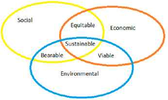
Visual description of sustainability

The evaluation of sustainability in transportation decision making has been practiced by different techniques, which are categorized in eight groups ⁶:

1. 1.

   Life-cycle analysis (LCA), which has limited applications in transportation decision⁷.

2. 2.

   Cost-benefit analysis (CBA) and cost effectiveness analysis (CEA) that address the monetary aspect of positive and negative effects of projects⁸.

3. 3.

   Environmental impact assessment (EIA), which is in a number of studies included in transportation evaluations⁹.

4. 4.

   Optimization models used for sustainable transportation¹⁰.

5. 5.

   System dynamics models that illustrate the relationships of the system elements by reviewing time-varying flows and feedback mechanisms¹¹.

6. 6.

   Assessment indicator methods that are subdivided among composite index models, multi-level index models, and multi-dimension matrix models ¹².

7. 7.

   The data analysis approach that applies statistical methods to assess sustainability.

8. 8.

   Multi-criteria decision analysis (MCDA) methods including some of the well-known techniques like analytic hierarchy process (AHP) and ELECTRE methods.

MCDA is the preferred approach for problems with conflicting objectives. Since the environmental, social, and economic aspects with their own measurement units can be aggregated in this approach, it is known as a reliable method for sustainable transport decision-making problems¹³. Tsamboulas¹⁴ used multiple attribute utility theory (MAUT) to rank transportation projects. Halouani et al.¹⁵ studied the aggregation of quantitative and qualitative information by introducing two multi-criteria group decision methods to select the right projects. The main difference of multi-criteria analysis (MCA) and CBA is the ability of MCA to use both qualitative and quantitative parameters while CBA just assesses monetized values indicating costs and benefits^16,17. Thus, MCA overcomes the disadvantages of assessing monetary values for aspects like noise pollution that are hard to ascertain¹⁸. Moreover, the MCA is increasingly being applied in transport decision making for several reasons, such as the complexity of the issues, the necessity to holistically address environmental, economic and social aspects, and the inadequacies of other methods like CBA in considering all the different aspects of a capital¹⁹.

Tudela et al.¹⁷ explored the results of CBA and MCA by comparing two alternatives in a part of the road system in Chile. The results showed that on a purely economic basis the same alternative was chosen by both methods. On the other hand, when non -economic and environmental aspects were considered, the techniques selected different alternatives. The alternative eventually regarded by the authority was the one chosen by the MCA approach while addressing environmental effects. Moreover, the impacts on the local community were severely underestimated while applying the CBA method.

MCDA methods are considered as the most common method applied in sustainable transportation evaluation. On the contrary, they seem inadequate while dealing with complexity, uncertainties and impreciseness that exist in almost all investment selection problems. In other words, all of the transport decisions are often made under imprecise and uncertain circumstances with partial and incomplete truth. A number of objectives and limitations are in many cases difficult to be measured by crisp values. Traditional analytical approaches were identified as non-effective in cases handling problems in which the dependencies between variables are too complicated or even in some cases ill-defined. Moreover, hard computing models cannot deal effectively with the transport decision-makers’ ambiguities and uncertainties. The first and the most important uncertainty is the aspects of uncertain demand. Another important source of uncertainty is related to the cost of investment¹⁸.

A variety of deterministic and stochastic methods has been developed over the years to address complex transportation problems. Those models applied different equations to solve such problems. Whereas while addressing real-life engineering problems, data is often in linguistic nature and it is often too complex to be easily quantified by classical mathematical techniques. A widely accepted tool to address uncertainty is fuzzy sets theory. Many scholars have used fuzzy sets theory to address uncertainty in project evaluation and selection problems^20–24. Over the years, a large number of fuzzy multi-criteria decision making (FMCDM) techniques have been developed that differ in areas such as the type of questions asked, theoretical background, and sort of obtained results^25–30. They are all mainly concerned with making the process better informed and structured.

Celik et al.³¹ used axiomatic design and TOPSIS methodologies to analyze competitive strategies on Turkish container ports in maritime transportation network. Tuzkaya³² developed an approach based on the concept of fuzzy AHP and the method of PROMETHEE I and II to evaluate the most environmental friendly way of transportation in the Marmara region, Turkey while considering all the concerned stakeholders. Awasthi et al.⁶ applied fuzzy TOPSIS to evaluate sustainable transport projects. Awasthi et al.³³ introduced a model based on affinity diagram, AHP and TOPSIS for sustainable city logistics planning under fuzzy uncertainty. Mandic et al.³⁴ proposed a two-phase model for multi-criteria project ranking with application in Serbian railway by applying fuzzy sets theory. Rossi et al.³ developed a method that applied fuzzy-based evaluation method (F-BEM) to evaluate sustainable transport policies.

Despite all the efforts to model uncertainty in MCA methods, most of the studies like the aforementioned studies were based on classical fuzzy sets. As fuzzy sets theory was more applied in real-world problems, its shortcomings made it crystal clear that it is essential to enhance fuzzy sets theory. One of classical fuzzy sets theory shortcomings happens when a decision maker (DM) is expected to express an exact opinion by a crisp number in interval [0, 1]. Therefore, in real situations and in uncertain environments expressing this degree of certainty by an interval is more suitable. This approach is supported by interval-valued fuzzy sets (IVFSs). By applying these sets, the DM can state unknown and vague membership degrees by replacing traditional [0, 1]-valued membership degrees by intervals in [0, 1]. If in a problem tangible facts or proofs did not exist and expressing lack of information and vagueness based on feelings was unavoidable, IVFSs could be the required tool to model uncertainty. Furthermore, IVFSs are considerably easier in application in comparison with type-2 fuzzy sets^35–37.

In this paper, a new approach of sustainable transportation investment selection is proposed that unlike most of the studies on this subject applies IVFSs to express and model uncertainty. Moreover, the proposed method is based on the concepts of relative preference relation on fuzzy numbers, the recently developed fuzzy TODIM (an acronym in Portuguese for Tomada de Decisão Interativa Multicritério meaning iterative multi-criteria decision making) and the importance weight of the decision makers. In other words, the proposed method extends the concepts of relative preference relation to interval-valued fuzzy (IVF)-numbers and applies it to determine the importance of sustainability criteria. Also, a new approach is proposed to address the weight of each expert’s opinion by considering all the gathered judgments and the importance of each expert in his/her especial area of expertise. Moreover, the criteria that depends on cost is addressed by developing benefit to cost analysis under an IVF-environment. Furthermore, the concept of TODIM is extended in an IVF-environment. TODIM is a global multi-attribute value function that is made in parts, with their mathematical descriptions reproducing the gain/loss function of a theory introduced by Kahneman and Tversky³⁸ and known as Prospect Theory. It should be noted that this theory was the basis of the Nobel Prize for Economics awarded in 2002^39,40. Aggregation of all measures of gains and losses over all criteria is carried out by the global multi-attribute value function of TODIM.

Finally, this paper proposes a new method for ranking IVFSs based on the concepts of ideal positive and ideal negative solutions. In summary, the main features of this paper that separate it from the similar studies in this area are as follows: (1) Due to importance of social and environmental impacts of transport projects, the concept of sustainability is considered in the decision-making process; (2) A new model of IVF-ranking is proposed based on the concept of ideal positive and ideal negative solutions; (3) Weight of each criterion is calculated by the principles of relative preference relation on IVF-numbers; (4) Weight of each expert is calculated by using a novel approach that not only considers expertise of each expert in his/her own area but also uses the average of the gathered data and the distance from the best and the worst opinion; and (5) TODIM is extended in an IVF-environment and is applied as a main step in the decision-making process to find the best sustainable transport project.

The rest of the paper is presented as follows. In section 2, the preliminary knowledge of IVFs is presented. In Section 3, the proposed methodology is introduced. In section 4, the method is applied in a case study, and the results are presented and discussed. Finally, section 5 concludes the paper.

2. Preliminary

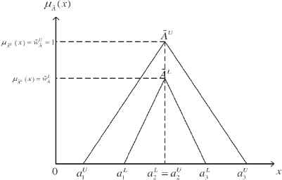
In the following, in order to provide preliminary knowledge of IVFSs, first the characteristics of triangular interval-valued fuzzy numbers are defined. Then, the arithmetic operations between two triangular IVF-numbers are presented. This section also includes a new ranking method for IVFs. The preliminary knowledge of IVFSs is presented as follows:

• A triangular interval-valued fuzzy number (shown in Figure 2) is characterized by Ã^L and Ã^U that denote the lower and upper triangular interval-valued fuzzy numbers, and W^A˜L and W^A˜U that express the degrees in which an event x could be a part of the lower and upper numbers, respectively⁴¹. This number can be depicted as:

  (1)A˜=[A˜xL,A˜xU]=[(a1L,a2L,a3L;wA˜L),(a1U,a2U,a3U;wA˜U)]

• Arithmetic operations between two triangular IVF-numbers à and B˜ expressed as A˜=[(a1U,a1L),a2,(a3L,a3U)] and B˜=[(b1U,b1L),b2,(b3L,b3U)] , respectively are presented as follows ^42,43.

  • Addition ⊕:

    (2)A˜⊕B˜=[(a1U,a1L),a2,(a3L,a3U)]⊕[(b1U,b1L),b2,(b3L,b3U)]      =[(a1U+b1U,a1L+b1L),a2+b2,(a3L+b3L,a3U+b3U)]

  • Subtraction ⊖:

    (3)A˜⊖B˜=[(a1U,a1L),a2,(a3L,a3U)]⊖[(b1U,b1L),b2,(b3L,b3U)]      =[(a1U−b3U,a1L−b3L),a2−b2,(a3L−b1L,a3U−b1U)]

  • Multiplication ⊗:

    (4)A˜⊗B˜=[(a1U,a1L),a2,(a3L,a3U)]⊗[(b1U,b1L),b2,(b3L,b3U)]      =[(a1U×b1U,a1L×b1L),a2×b2,(a3L×b3L,a3U×b3U)]

  • Generalized division ⊘:

    (5)A˜B˜=[(a1U,a1L),a2,(a3L,a3U)][(b1U,b1L),b2,(b3L,b3U)]=[(a1U÷b3U,a1L÷b3L),a2÷b2,(a3L÷b1L,a3U÷b1U)]
    where b1L , b₂, b3L , b3U are non-zero positive real numbers.

Figure 2.

An interval-valued triangular fuzzy number A˜(W^A˜L≠W^A˜U)

3. Introduced multi-criteria analysis approach

In this section, first, the evaluation criteria are defined and then how they are addressed in the proposed approach is described. Then, the IVF-based sustainable evaluation method is presented.

In order to effectively select and define the sustainable evaluation criteria in this paper, a careful review of some of the recent studies on this subject (i.e., Shiau¹³; Salling and Pryn⁴⁸; Geurs et al.⁴⁹; Véron-Okamoto and Sakamoto⁵⁰; Awasthi et al.⁶) was carried out. As a result, the evaluation criteria are divided into two main groups of monetary and non-monetary. Non-monetary criteria are addressed by obtaining the judgments from the experts. For monetary criteria, a different approach is presented. In order to address the cost benefit analysis of these criteria, since B/C method presents a comprehensive index¹³, in this paper, the concept of B/C analysis is extended to an IVF-environment and the following is presented:

From a different perspective, the evaluation criteria are divided into groups of economic, social and environmental criteria. The evaluation criteria with a brief description are presented in Table 1.

3.1. Introduced compromise ratio model

In this sub-section, a compromise ratio method that is based on the concepts of IVFSs, relative preference relation, TODIM and the weights of each decision maker is introduced to address sustainable criteria in transportation decision making. Moreover, this systematic process avoids information loss while considering the weights of decision makers (DMs). After normalizing the decision matrix, a weight is given to importance of each criteria by using fuzzy preference relation. Then, a process is developed to compute weight of each decision maker and eventually, the weights computed for importance of criteria and decision makers are applied in the evaluation and ranking process. Linguistic variables were converted into IVFSs to address criteria values and criteria weights. These converted values are presented in Tables 2 and 3⁵¹. Applying IVFSs provides the DM with more flexibility in expressing lack of knowledge and vagueness when difficultie s in expressing the membership degrees by a crisp value arise. The introduced method of decision making is described in detail as presented:

Linguistic variables	IVF-numbers
Very poor (VP)	[(0,0),0,(1,1.5)]
Poor (P)	[(0,0.5),1,(2.5,3.5)]
Moderately poor (MP)	[(0,1.5),3,(4.5,5.5)]
Fair (F)	[(2.5,3.5),5,(6.5,7.5)]
Moderately good (MG)	[(4.5,5.5),7,(8,8.5)]
Good (G)	[(5.5,7.5),9,(9.5,10)]
Very Good (VG)	[(8.5,9.5),10,(10,10)]

Table 2.

Linguistic terms for ratings

Linguistic variables	IVF-numbers
Very Low (VL)	[(0,0),0,(0.1,0.15)]
Low (L)	[(0,0.05),0.1,(0.25,0.35)]
Medium Low (ML)	[(0,0.15),0.3,(0.45,0.55)]
Medium (M)	[(0.25,0.35),0.5,(0.65,0.75)]
Medium High (MH)	[(0.45,0.55),0.7,(0.8,0.85)]
High (H)	[(0.55,0.75),0.9,(0.95,1)]
Very High (VH)	[(0.85,0.95),1,(1,1)]

Table 3.

Linguistic terms for the importance weight of each criterion

At the beginning of the introduced process, judgments of every one of the DMs should be obtained. As a result, the followings are gathered:

(11)R˜K=(R˜ijK)m×n=[R˜11K⋯R˜1nK⋮⋱⋮R˜m1K⋯R˜mnK]

(12)W˜k=(w˜1k,w˜2k,…,w˜nk),K∈T

Where R˜K is the decision matrix and W˜K is the weight vector of attributes, m denotes the number of criteria and n shows number of compared alternatives and T shows the group of experts. w˜j is the weight vector of the criteria. It should be considered that since R˜ijK and W˜K are IVFSs, they are denoted as follows:

R˜ijK=[(rij1U,rij1L),rij2,(rij3L,rij3U)]

W˜K=(wj1U,wj1L),wj2,(wj3L,wj3U)

The normalized decision matrix (G˜) presented in Eq. (15) is calculated by applying Eqs. (16) and (17). In order to make different criteria comparable, normalization process is carried out. To put differently, normalization makes dimensionless values of different criteria.

(15)G˜=[G˜11⋯G˜1n⋮⋱⋮G˜m1⋯G˜mn]

(16)G˜ij=[((rij1Ur*),(rij1Lr*)),(rij2r*),((rij3Lr*),(rij3Ur*))]      i=1,2,…,n,j∈B

(17)G˜ij=[((r−rij3U),(r−rij3L)),(r−rij2),((r−rij1L),(r−rij1U))]      i=1,2,…,n,j∈C

Where B denotes the set of benefit criteria and C represents the set of cost criteria. r^* and r⁻ are also obtained as presented in Eqs. (18) and (19):

(18)r*=maxi(rij)3U

(19)r−=mini(rij)1U

In order to compute relative preference degrees of the IVF important levels over the IVF average values, first the average of the values for importance of criteria should be calculated. The calculation is presented as follows in Eq. (20):

(20)W˜¯j=((∑k=1Twjk1UT,∑k=1Twjk1LT),∑k=1Twjk2T,(∑k=1Twjk3LT,∑k=1Twjk3UT))

In this Eq., W˜¯j denotes the average of values expressing importance of criteria.

The relative preference relation (RPR), categorized by its membership function μRPR(Wkj,W¯j) , determines the relative preference degree of W_kj over W¯j . It is calculated as follows in Eqs. (21) and (22):

(21)μRPR(Wkj,W¯j)=12((wtj1U−∑k=1Twjk3UT)+2(w˜tj2−∑k=1Twjk2T)+(wtj3U−∑k=1Twjk1UT)2||Pw||+1)

Where ‖P_w‖:

(22){(pw+1U−pw−3U)+2(pw+2−pw−2)+(pw+3U−pw−1U)2,ifpw+1U≥pw−3U(pw+1U−pw−3U)+2(pw+2−pw−2)+(pw+3U−pw−1U)2+2(p¯w3U−pw+1U),ifpw+1U<pw−3Upw+1U=maxKwkj1U,pw+2=maxKwk˙j2,pw+3U=maxKwkj3U,pw−1U=minKwkj1U,pw−2=minKwkj2.,pw−3U=minKwkj3U

Finally, the weights of criteria are given a value denoting their importance based on the concept of the relative preference relation. The new weights (NW) of criteria are calculated as follows in Eq. (23):

(23)NWj=μRPR(Wkj,W¯j)×Wj

The computed value in Eq. (23) is used in the Eq. (38). The normalized weighted decision matrix, presented in Eq. (24), is calculated by employing Eq. (25).

(24)F˜=[F˜11⋯F˜1n⋮⋱⋮F˜m1⋯F˜mn]

(25)F˜ij=G˜ij×w˜j=[((gij)1U×(wj)1U,(gij)1L×(wj)1L),(gij)2×(wj)2,((gij)3L×(wj)3L,(gij)3U×(wj)3U)]

The average of all individual decisions denotes the ideal decisions of all individual judgments in mean sense. A negative ideal decision is with the maximum separation from the positive ideal decision. Therefore, the left negative ideal decision and right negative ideal decision are obtained⁵². Thus, the best judgment (F^*), the left negative ideal judgment (Fl−) and the right negative ideal judgment (Fr−) are computed by employing Eqs. (26), (27) and (28), respectively:

(26)F˜*=[F˜*11⋯F˜*1n⋮⋱⋮F˜*m1⋯F˜*mn]

where F˜*ij=[(/t1∑k=1tfij1U,/t1∑k=1tfij1L),/t1∑k=1tfij2U,(/t1∑k=1tfij3L,/t1∑k=1tfij3U)]

(27)F˜L−=[F˜l−11⋯F˜l−1n⋮⋱⋮F˜l−m1⋯F˜l−mn]

where F˜l−ij=min1≤k≤t{F˜ijk}

(28)F˜R−=[F˜r−11⋯F˜r−1n⋮⋱⋮F˜r−m1⋯F˜r−mn]

where F˜r−ij=max1≤k≤t{F˜ijk} The separations of each individual decision from the ideal decisions including positive ideal decision, the left negative ideal decision and the right negative ideal decision are respectively denoted by ok* , olk− and ork− , and they are computed by applying Eqs. (29), (30) and (31), respectively:

(29)ok*=16∑p=13((fijpUk−fijpU*)2+(fijpLk−fijpL*)2)k∈T

(30)olk−=16∑p=13((fijpUk−fijpUl)2+(fijpLk−fijpLl)2)k∈T

and

(31)ork−=16∑p=13((fijpUk−fijpUr)2+(fijpLk−fijpLr)2)k∈T

The closeness coefficient of the individual decision with respect to ideal decisions denoted by IC_k is presented as follows in Eq. (32):

(32)ICk=olk−+ork−olk−+ork−+ok*,K∈T

Obviously larger value of IC_k shows more importance on kth DMs judgments, and heavier weight for kth DM⁵³. It should be considered that the relative importance of each DM is measurable and quantifiable. Consequently, the importance of an expert in his/her area of expertise called the individual importance is displayed by II_k. To have a DM weight that considers both of the aforementioned aspects, the aggregated form is presented in Eq. (33) as follows:

(33)AWk=βIIk+(1−β)ICk,K∈T

Where β(0 ≤ β ≤ 1) is the optimistic coefficient that indicates whose value can be chosen according to group’s opinion, II_k (0 ≤ II_k ≤ 1) is the measure of importance of kth DM as an expert in his/her own area of expertise.

Eventually, the weights of DMs are obtained in Eq. (34) as follows:

(34)DMWk=AWk∑k=1tAWk,K∈T

The weighted (on attributes and DMs) decision matrix (H) for each DM is calculated by the following in Eq. (35):

(35)H˜k=(hij)m×n=(DMWk×fijk)m×n=[H˜k11⋯H˜k1n⋮⋱⋮H˜km1⋯H˜kmn]

where H˜ij=[(dmwk×(fj)1U,dmwk×(fj)1L),dmwk×(fj)2,((fj)3L×dmwk,(fj)3U×dmwk)]

The conventional multi-attribute group decision-making problems are characterized by three items: alternative, attribute and DM. Up to this point of the proposed method, the focus of the approach was on DM. To rank the preference order of alternatives, the focus will be shifted on the alternative.

The weighted (on attributes and DMs) individual decision is converted into the group decision, for each alternative. This is done by the following in Eq. (36):

(36)H˜i=(Hkj)j×n=[H˜i11⋯H˜i1n⋮⋱⋮H˜it1⋯H˜itn],i∈M

The dominance of each alternative Ã_i over each alternative Ã_j is calculated by using Eqs. (37) and (38):

(37)ϑ(A˜i,A˜j)=∑c=1mψc(A˜i,A˜j),∀i,j

(38)ψc(A˜i,A˜j)={d(NWrc)d(Σc=1mNWrc).16∑p=13((hicU−hjcU)2+(hicL−hjcL)2),if hic>hjc0,if hic=hjc−1θd(Σc=1mNWrc)d(NWrc).16∑p=13((hicU−hjcU)2+(hicL−hjcL)2),if hic<hjc

ψ_c(Ã_i, Ã_j) shows the contribution of the criterion c to the function ϑ(Ã_i, Ã_j) while comparing Ã_i with Ã_j.

The value NW_rc represents the weight of criterion c divided by the weight of the criterion that has the biggest weight. The term d denotes the distance of the fuzzy ratings. Three situations can happen in Eq. (38): h˜ic>h˜jc shows gain, h˜ic=h˜jc denotes zero which means neither gain nor loss and h˜ic<h˜jc represents loss. The attenuation factor of the losses is denoted by θ. Different values lead to different shapes of the prospect value function in the negative quadrant as depicted in Figure 3 ⁵⁴. The partial matrices of dominance for each criterion are summed up to form the final matrix of dominance.

Figure 3.

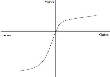
Prospect value function.

Eventually Eq. (39) is applied to normalize the final matrix of dominance and calculate the global value of the alternative i.

(39)τi=∑ϑ(i,j)−min∑ϑ(i,j)max∑ϑ(i,j)−min∑ϑ(i,j)

The final ranking of each alternative is obtained by sorting the values of τ_i in decreasing order. The best alternative has the highest value τ_i.

4. Case study

In this section in order to explain the applicability of the proposed sustainable transport investment evaluation approach in real-world problems, the proposed method is used in a real case study of an Iranian transport complex. The main objective of company is to bring integration and multi-aspect transportation services inside the country and overseas in areas such as marine, rail, road and air transportation. Moreover, their goal is to become one of the most efficient integrative transportation complexes inside the country within the coming five years in areas such as productivity, operational capability, and market portion and development capacity. Some of the main areas that the company has its focus on includes: Oil products transit, replacement of different types of liquids and fuel inside and outside the country, presenting technical, engineering services, and executing industrial projects in marine and rail sectors, importing and exporting, purchase and sale all required feasibilities for marine industries, refinery, petrochemical and its transportation, performing all marine & port services, drainage, tugboat, loading and offloading of oil and non-oil products, presenting container terminals services.

The company is presented with four alternative transport investments. Due to the limited investment funds, the company wants to choose the best one of the projects to fund and operate. Their main goal is to improve their position inside the country through enhancing the existing project conditions by focusing on issues, such as clean technology development and sustainability. Due to the competitive environment, the company has reserved the information of candidate projects as confidential. Due to confidentiality of the information, limited details of the projects are presented.

Four candidate investment projects denoted as A₁, A₂, A₃ and A₄ have the following features. A₁ is a marine transport project aimed at European markets. This project involves using new transport project technologies and modern vessels. The route is from Iranian ports in Persian Gulf to European markets. Figure 4 displays the Iranian ports in Persian Gulf. A₂ is a marine project that uses older vessels for Asian markets. A₃ is a marine transport project that is aimed at Caspian sea and Black sea markets. Finally, A₄ is a road transport project aimed at Caucasus region. Figure 5 displays the Caucasus region countries.

Figure 4.

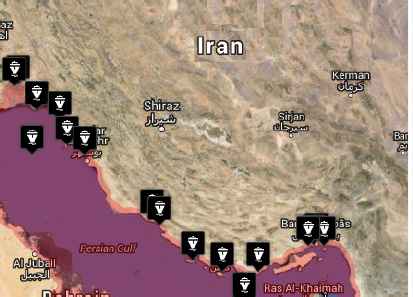
Iranian ports in Persian Gulf

Figure 5.

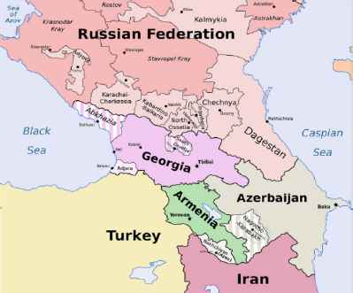
Caucasus region

In order to apply a more flexible tool to address uncertainty, IVFSs were used to describe projects. Furthermore, the knowledge of experts were used to distinguish the relative importance of proposed criteria of sustainable project selection. Thus, a group consisting of 3 experts with at least 15 years of experience in transport sector was formed. Questionnaires were used to gather data from experts of the aforementioned company. Due to the available data and the fact that the investments were at the proposal phase, return on investment was considered as a quantifiable monetary criteria and the rest were directly expressed by experts’ judgments. Tables 4 and 5 displays the information considering return on investment.

Table 6 provides the decision matrix, and Table 7 expresses the weight vector of attributes (criteria). It should be noted that in this section, the evaluation criteria are stated as cost or benefit criteria. The benefit criteria consists of C₁ (return on investment), C₃ (reduction in costs), C₄ (safety), C₅ (affordability), C₆ (employment), C₇ (basic accessibility), C₈ (greenhouse gas emissions), C₉ (climate and global warming) and C₁₀ (resource efficiency). The cost criteria includes C₂ (financial risk). Projects are denoted as A₆, A₂, A₃ and A₄, and experts are referred to as E₁, E₂ and E₃.

Since C₁ is a monetary criterion, Eq. (10) is used to assess them. The DMs have set the value of i equal to 0.05%. Table 8 displays the financial assessments of the alternatives.

The financial analysis results were given to the experts and they were asked to express their judgments of project evaluation for C₁. Table 9 displays the outcome.

Eqs. (16) and (17) are used to normalize the decision matrix. Eq. (20) is used to compute the average of the values for importance of criteria. The results are displayed in Table 10. Eqs. (21)– (23) are used to calculate the new weights of criteria. The results are displayed in Table 11.

The normalized weighted decision matrix is computed by using Eq. (25).

The best judgment (F^*) is computed by using Eq. (26). The left negative ideal judgment (Fl−) and the right negative ideal judgment (Fr−) are also identified by using Eqs. (27) and (28). The results are presented in Table A1. This table is presented in appendix.

For the next step, it is necessary to compute the values of ok* , olk− and ork− by using Eqs. (29)– (31), respectively. The results are presented in Table A2, given in appendix.

IC_k is computed by applying Eq. (32). Then AW_k is obtained by using Eq. (33). It should be noted that after discussing the model with the decision makers β was considered as 0.25 and II_k was considered as 0.3 for each DM. Finally, the weights of DMs are obtained by using Eq. (34). Table A3, given in appendix, displays the values of IC_k, AW_k and DMW_k.

The weighted (on attributes and DMs) individual decision is gained by using Eq. (35). Then, it is converted into the group decision, for each alternative by applying Eq. (36). Dominance of each alternative Ã_i over each alternative Ã_j is computed through using the Eqs. (37) and (38). θ denotes the attenuation factor of the losses. In other words, if the DMs are willing to ignore the impacts of losses and focus more on the wins, they will give values bigger than 1 to θ. If the value of θ is set as 1, it means that losses will contribute with their real value to the global value. From the risk acceptance perspective, it can be argued that bigger values of θ mean that the DMs are more willing to welcome risk in their decision making. However, smaller values of θ (especially less than one) denote that the DMs are more worried about losses and focus more on them. In the literature, often small values are given to θ (e.g., Liu and Teng⁵⁵; Krohling et al.⁵⁶; Gomes⁴⁰). In the studied case, the DMs as professional experts in this area were willing to give a high value of attenuation factor to losses. In other words, they wanted to pay more attentions to wins. Therefore, after reviewing the preference of the DMs, the value of 15 was chosen for the attenuation factor. This value denotes an upper bound for θ meaning that bigger values would not reflect the preference of the DMs. However, in the sensitivity analysis section, values of 10, 5, 2.5 and 1 are also given to the attenuation factor to investigate the impact of lower values on the final decisions. Table 12 displays the results of ∑ϑ(i,j) .

Finally, in order to rank the alternatives, Eq. (39) is used. The results are displayed in Table 13. In order to explore the robustness of the model, θ was changed to 5 and 10. The results show that the ranking stays intact. As it can be seen, project A₁, marine transport project for European markets using modern vessels, has the best score. Then, projects A₃ and A₂ have the best outcomes, respectively. Finally, A₄ has the worst ranking.

In order to validate the results, the decision method of Ashtiani et al.⁴⁶ for IVFSs was applied in the case study. The results are presented in Table 14. This table presents the values of RC₁, RC₂ and RCi* . These values denote the relative closeness for the lower (RC₁) and the upper (RC₂) number. The final value (RCi*) is the outcome of aggregation of the lower and the upper numbers. As it can be observed in this table, the ranking stays intact for all alternatives. The presented method is similar to the method of Ashtiani et al.⁴⁶ in case that both apply IVFSs to rank alternatives. However, the presented method has the following advantages over the method of Ashtiani et al.⁴⁶: (1) The DMs are given a weight based on their expertise and the gathered judgments. This method avoids information loss in computing weights of the DMs; (2) the developed method applies the relative preference relation to further address the weight of criteria; and (3) the applied method uses the prospect value function to rank the alternatives.

5. Conclusion

Sustainability has become an important part of any development plan. When it comes to transportation, this issue becomes more critical. On the other hand, uncertainty is an important factor in any decision making process under real-world conditions. In this paper, a novel compromise decision-making process was introduced that used interval-valued fuzzy sets (IVFSs) to model uncertain environment of transport investment projects. The model used the concept of fuzzy relative preference to address weight of selection criteria. Moreover, a new process was applied to compute the weight of decision makers in the process based on the knowledge of the experts and the gathered judgments. This last aggregation based model would avoid loss of information. Moreover, the concept of Prospect theory was applied in the model through extending the existing knowledge of TODIM to IVF-environment. Finally, to show the applicability of the proposed model, real data from an Iranian transport was adopted and used in the case study. In that section, four different transport projects were step by step evaluated through monetary and non-monetary criteria. Finally, the results were presented, and a sensitivity analysis on one of the parameters was carried out. Despite showing the interaction of opinions on ratings and criteria weights in the process, the interaction of criteria on each other was not fully addressed in this paper. To the best of our knowledge, this impact has been ignored in most of the studies and considering this impact could provide an interesting future research direction.