
Empirical Comparison of Differential Evolution Variants for Industrial Controller Design
- DOI
- 10.1080/18756891.2016.1237193How to use a DOI?
- Keywords
- Performance Measures; Differential Evolution Variants; Fixed-order Structured Controller; Model Matching; Optimization; Statistical Comparison
- Abstract
To be cost-effective, most commercial off-the-shelf industrial controllers have low system order and a predefined internal structure. When operating in an industrial environment, the system output is often specified by a reference model, and the control system must closely match the model’s response. In this context, a valid controller design solution must satisfy the application specifications, fit the controller’s configuration and meet a model matching criterion. This paper proposes a method of solving the design problem using bilinear matrix inequality formulation, and the use of Differential Evolution (DE) algorithms to solve the resulting optimization problem. The performance of the proposed method is demonstrated by comparing a set of ten DE variants. Extensive statistical analysis shows that the variants best/1/{bin, exp}and rand-to-best/1/{bin,exp}are effective in terms of mean best objective function value, average number of function evaluations, and objective function value progression.
- Copyright
- © 2016. the authors. Co-published by Atlantis Press and Taylor & Francis
- Open Access
- This is an open access article under the CC BY-NC license (http://creativecommons.org/licences/by-nc/4.0/).
1. Introduction
Traditional control design requires a full order controller: the order of the controller must always be greater than or equal to the dimension of the process model. This can be a severe restriction, especially when the process model dimension is high and the controller is an embedded device with limited memory and processing power. Moreover, traditional design techniques are unable to take into account the fixed structure of commercially available controllers, such as the popular PID (proportional, integral, derivative) feedback compensator. For the class of control problems that minimize a model matching criterion, a specific model is given and the design of the controller has to ensure that the compensated process meets the specific model’s behavior. If the controller’s structure is fixed, then the problem becomes one of finding its gains while minimizing the model matching error. Consequently, the design of low-order and fixed structure controllers with a model matching criterion poses a challenging problem with many practical consequences. Fortunately, the problem can be reformulated as a bilinear matrix inequality (BMI) problem, with linear matrix inequality (LMI) subproblems associated to the lower and upper bound estimations. The resulting non-convex problem can be solved by the application of a branch and bound (BB) algorithm. Although BB is known to be optimal, it also has a very slow convergence speed.1 Therefore, determining an effective alternative solution method is an ongoing research subject.
The differential evolution (DE) algorithm is a well-known population-based evolutionary optimizer designed for real-valued optimization purposes. Note that for simplicity’s sake we will use “DE” to refer to “differential evolution algorithm” throughout this paper. A DE has four controlling parameters: the mutation factor (F), the crossover probability (CR), the population size (NP), and the maximum number of generations (gmax). There are at least ten basic variants, and new variants and extensions are constantly being developed by researchers.2 The aim here is to propose an evaluation procedure that can determine which DE variants are suitable as alternatives to the BB algorithm.
From a practical point of view, the outcome of an evaluation procedure should accurately indicate the set of DE optimizers that are effective for the particular engineering problem at hand. This indication is usually deduced from measurements made during and after algorithm executions. These measurements should cover both the efficacy and efficiency of the DEs. Here, “efficacy” is the ability to produce a desired result, and “efficiency” is the ability to produce a desired result with minimum wasted effort. Obviously, it is best to seek out DEs that are both efficacious and efficient. Since DEs are stochastic optimizers, the measurements are random variables and multiple trial runs are needed to estimate their underlying statistics. Thus, the relevant statistics are presented along with their confidence intervals, and conclusions are inferred by statistical tests.
The outline of this paper is as follows. Section 2 surveys recent experimental work on DE, with emphasis on the comparable methodological elements. Section 3 reviews different DE variants and their operating principles. Section 4 formalizes the non-convex optimization problem resulting from a BMI formulation of a structured controller with a matching model criterion. Section 5 details the performance measures and setup used during the experiments. Section 6 provides an extensive statistical analysis of the obtained results. Section 7 concludes the paper.
2. Related Works
Empirical comparison is a methodology of applied inductive research and development. Its goals are to discover knowledge through experimentation, to develop efficient solutions for a specific environment, and to validate performance claims.3 Thus, an empirical comparison should have a stated goal, a reproducible experimental setting, a set of performance measures, and an explicit data analysis procedure. Each of these elements contributes to the inductive process that leads to the drawing of conclusions. This is the perspective adopted in the brief review of literature that follows.
In Ref. 4, Mezura-Montes et al. compared eight DE variants on 30 test functions with known optimal values. The DE parameters included a range of values for the mutation factor F ∈ [0.3, 0.9], the crossover probability CR ∈ {0.0,0.1,0.2,…,1.0}, the population size NP = 60, the maximum number of generations gmax = 2000, and the total number of trial runs NT = 100. The reported performance measures are the mean best objective function values
To take into account unsuccessful trial runs, Auger et al.5 divided the average number of evaluations for successful runs by the ratio of successful runs to the total number of trial runs. They considered two deterministic optimization algorithms: BFGS (Broyden–Fletcher–Goldfarb–Shanno quasi-Newton method), and Powell’s NEWUOA trusted region method. These algorithms were each compared with a DE variant (local-to-best/1/bin), CMA-ES (Covariance Matrix Adaptation Evolution Strategy), and PSO (Particle Swarm Optimization) on three test functions. Each of these optimization algorithms has its own set of controlling parameters. Auger et al. ran NT = 21 independent trials with a maximum of 107 function evaluations for each of the test functions. Part of their results showed that NEWUOA outperformed all other algorithms on the separable Ellipsoid function up to a condition number of 106. The BFGS method performed better than PSO and CMA-ES, and the DE variant showed the worst performance. Although this multi-algorithm comparison is thoroughly comprehensive, it is difficult to make use of the findings because no relevant statistical measures were reported in their wok.
In part of Ref. 6, Jeyakumar and Shanmugavelayutham investigated the convergence nature of fourteen DE variants with fourteen test functions in 30D. They used gmax = 3000 and NT = 100, and the same values for NP, F and CR ranges as Ref. 4. They also adopted the same performance measures used in Ref. 5, with the addition of a population diversity measure defined as the Euclidean distance between the center of a population and its farthest individual.7 The performance measures are given in terms of mean, standard deviation and variance. This is a methodological improvement compared to the preceding works; however, they based their observations on numerical inspection without statistical testing.
More recently, Sacco et al.8 applied DE optimization to a nuclear core design problem. They compared the performance of two DE extensions: trigonometric mutation and opposition-based learning. Both algorithms were given the same NP, F and CR. They found that the opposition-based learning DE seemed to be more consistent and robust than the trigonometric mutation one. Here, the same set of parameter values should provide fairness and objectivity in the comparison procedure, but their conclusions were also based on simple numerical inspection.
Instead of relying on direct numerical comparison, Li et al.9 used the Wilcoxon rank-sum test to compare two new DE extensions, based respectively on covariance matrix adaptation and cumulative learning evolution (JADEEP and rand/1/EP), against their original variants on twenty-eight test functions of 30D, 50D and 100D. The Wilcoxon rank-sum test is also a nonparametric test, but the null hypothesis is that paired samples come from the same population. Since the Wilcoxon rank-sum test is designed for two related samples, it suffices to compare each DE extension to its original DE variant. Similarly, Fan et al.10 studied self-adaptive crossover and mutation strategies using 25 test functions and five DE variants. Their experimental setting included NT = 30 independent runs, NP = 50, and gmax = 1000. In their work, they applied the improved DE variants to estimate the kinetic parameters of a mercury oxidation model. Fan et al. highlighted the differences between the simulation and the actual values with graphical error bars. They also applied the Wilcoxon rank-sum test to compare the DE variants and the corresponding improved versions. Unfortunately, the Wilcoxon rank-sum test is only appropriate when testing two DEs, of which one may be an extension or an improved variant.
In order to compare more then two DEs, Apolloni et al.11 made use of Friedman’s rank test and post hoc Holm’s correction to compare three variants of distributed DE on test functions of dimensions 100 and 500. Friedman’s rank test is a non-parametric version of ANOVA, with data grouped in categorical factors or repeated measurements. In this case the factors are the test functions’ dimensions. If the null hypothesis (no difference between the groups) is rejected, it is necessary to perform post hoc tests to find out which of the DE variants are different. Holm’s correction is used in this context to control rejection errors. Olguin-Carbajal et al.12 also applied the Friedman and post hoc tests to compare a micro DE with only five candidate solutions (NP = 5), an adjusted DE for high problem dimensionality, and a standard DE variant (rand/1/bin) using the same F for all algorithms. Both of these works performed extensive empirical comparisons. However, they both limited their experiments to the use of a single performance measure, namely the average difference between DE fitness values and the test function’s optimal values.
In light of the preceding discussion, efficacy and efficiency performance measures and appropriate statistical analysis are needed to determine the effectiveness of the DE variants.
3. Differential Evolution and its Variants
Like other evolutionary algorithms, DE’s main evolutionary operations are mutation, crossover and selection. The main difference between a DE and, for example, a standard genetic algorithm is that in the DE, the difference between two candidate solutions produces a difference vector to explore the search space. And whereas other advanced algorithms, such as interactive genetic algorithms, include a provision for human decision-making in the evolution process,13,14 DEs apply the usual evolution operations to generate new candidate solutions. In DEs, mutation and crossover operations are responsible for search space exploration and the selection procedure provides the exploitation properties for the algorithm. Conceptually, the perturbation of a candidate solution, by mutation and crossover, is done by probabilistically replacing it with another solution. The latter is created by adding, to a randomly selected candidate solution, a change that is proportional to the difference between two other randomly selected solutions. Then the selection is done by a competition between the parent and its offspring. That is, the better of the two solutions moves on to the next generation.
Let D be the number of decision variables and NP the number of candidate solutions in the population. The candidate solution population at the g-th generation can be written as
Similarly, the crossover operation incorporates the current solution
Another commonly used DE crossover operation is to first choose an integer n with a discrete uniform distribution over the set {1,2,…,D}. This integer acts as a starting point in the current target solution
3.1. Basic DE Variants
The identification scheme referencing the different DE variants is fairly consistent.2,7 A basic DE descriptor is a triplet s/1,2/{bin, exp} where the first two elements describe the mutation type and the last element indicates the crossover type. In this descriptor, is the source vector for perturbation from the current population. Therefore, s= best means using the best candidate solution, s= rand signifies a candidate solution is randomly chosen by the algorithm, and s = rand-to-best is a combination of s = rand and s = best. The second element {1,2} denotes the number of weighted difference vectors used in the mutation operation. The last element {bin, exp} indicates whether the type of crossover is binomial (as in Eq. 2 ), or exponential (as in Eq. 3 ).
3.1.1. best/1/{bin, exp}
These variants use the best candidate solution in the current population, and one weighted difference vector for mutation. In this operation, two randomly selected candidate solutions are needed, such that
3.1.2. rand/1/{bin, exp}
These variants use a random candidate solution in the current population, and one weighted difference vector for mutation. In this operation, three randomly selected candidate solutions are needed, such that
3.1.3. rand-to-best/1/{bin, exp}
This mutation operation uses the best candidate solution as well as two randomly selected candidate solutions in the current population, such that
3.1.4. best/2/{bin, exp}
This mutation operation uses the best candidate solution in the current population and one weighted difference vector. There are four randomly selected candidate solutions involved, where
3.1.5. rand/2/{bin, exp}
These variants use a random candidate solution in the current population and one weighted difference vector for mutation. A total of five randomly selected candidate solutions are needed, and
In summary, the basic crossover operations are formulated in Eqs. 2 –3 . Eq. 4 describes the selection operation, which is the same for all DE variants. Finally, Eqs. 5 –9 define the different mutation operations.
4. Controller Design Problem
Continuous linear time-invariant feedback control systems are generally characterized by a plant, sensors, and a feedback controller. In this work, it is assumed that the controller is structured (a constraint on the form of the controller) and has a fixed order. The gain adjustment that minimizes the difference between a reference model and the closed loop of the feedback control system results in a non-convex optimization problem. The block diagram corresponding to this system is illustrated by Fig. 1.
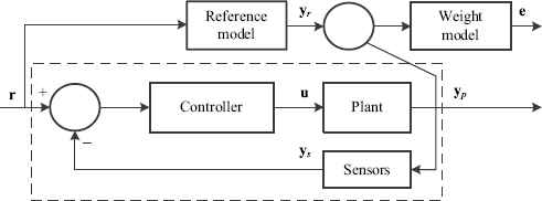
Block diagram of the feedback control system including a reference model and a weight model.
Note that there exists a weight error model between the reference model and the closed loop system, which provides a more flexible control system. In Fig. 1 the reference model is described in state-space form by
4.1. Minimization Problem
For the closed loop system described by Eq. 16 , the goal is to find the controller gain vector k that minimizes the error e. This optimization problem can be formulated as
5. Performance measures and experiment settings
As presented in Section 2, comparison reports using various performance measures are typical in the literature. Depending on their intent and design, performance measures can be computed during the DE’s trial run, after a trial run, or after all trial runs are completed. Several of these measures evaluate the DE’s ability to find an optimal solution. In practice, finding an optimal solution requires appropriate computation resources. Thus, there exist performance measures that are used to gauge the required computation resources for the DE to achieve its goal. The following subsections define and classify the performance measures related to this work.
5.1. Efficacy Measures
Let f* be the best known objective function value of a problem, Oi the best objective function value found by a DE variant during the i-th trial run, and
It is often useful to measure a DE’s optimization effort over time. This dynamic information can provide hints as to the convergence characteristics of an algorithm. A DE’s optimization effort can be measured by its output, or by
5.2. Efficiency Measures
For all successful trial runs, the average number of objective function evaluations,
Lastly, it is possible to combine an efficiency measure with an efficacy measure to obtain a hybrid measurement. The Q-measure is designed to produce a scalar indicating the quality of a DE. As defined in Ref. 7, the Q-measure is the number of objective function evaluations divided by the DE’s success ratio,
5.3. Statistical tests
The performance data generated by a DE variant are essentially samples taken from random variables with unknown distributions. To verify this affirmation in practice, all samples are subjected to the Shapiro-Wilk’s test for normality.15 Its null hypothesis is that the performance data sample is from a population with normal distribution. If the null hypothesis is rejected, statistics of performance measures are then estimated by using the bootstrap re-sampling method. To provide further information on the estimation, its 95% confidence interval (CI) is estimated by the bootstrap bias-corrected and accelerated method (BCa). The BCa confidence interval is a percentile method adjusted for the skewness in the bootstrap sampling distribution.16 When not overlapping, the CIs can be used to determine the mean difference between two samples. However, overlapping CIs do not indicate anything that is statistically significant.17 So, to compare DE performances, the Kruskal-Wallis rank test (or nonparametric one-way ANOVA test) with a 5% significance level is conducted in order to accept or reject the hypothesis that the mean ranks of the groups are the same, i.e., that the samples produced by the DE variants are the same for a given performance measure. It is important to select a statistical test that accounts for unequal sample sizes (when not all trial runs are successful) and to be able to test for several unmatched samples at once (since there are ten DE variants). If the null-hypothesis is rejected, then an all-possible pairwise comparison with Dunn-Sidàk significance level correction is applied to determine which DE variants are different. Dunn-Sidàk correction is known to be conservative under a dependence assumption, meaning that the actual corrected significance level is less than the prescribed 5% level.
5.4. Parameter settings
All trial runs are executed using MATLAB 8.4 on a 3 GHz PC computer. The best known controller gains (k*), and hence the best known objective function value f* are first obtained by a BB algorithm applied to the structured controller design problem instance that is specified in Fig. 2.
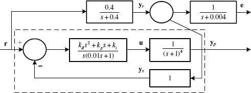
An instance of the structured controller design problem.
In this problem instance, the controller has an imposed PID structure and the plant has a higher order than both the controller and the reference model. It took BB global search 54400 objective function evaluations to obtain k* =[0.38940428 1.2219238 2.1276856]⊤ and f* = 0.0489462. The DE parameters and experiment variables are summarized in Table 1 and Table 2. In Table 1, D, (xL,xU), NT, NP and gmax are DE controlling parameters. The same values are used for all ten variants. The best known objective function value f* is obtained by a BB algorithm, and ∈ determines the closeness tolerance of an objective function value to f*. The population size NP, mutation factor F, and crossover rate CR are taken from numerical suggestions found in Ref. 2 and Ref. 18, and are manually tuned to one significant digit. The mutation factor and crossover rate are replaced by 1−F and 1−CR for DE variants that were unable to reach the vicinity of f* during initial testing. Each DE variant has NT = 100 trial runs with gmax = 100. The aim is to determine, using these experiment settings, which of the ten DE variants is capable of solving the proposed problem instance efficaciously and efficiently.
| Parameter | Value |
|---|---|
| Problem dimension | D = 3 |
| Decision var bounds | xL =[000]⊤,xU =[101010]⊤ |
| Nb of trials | NT = 100 |
| Population size | NP = 20 |
| Max nb of generations | gmax = 100 |
| Best known obj value | f*= 0.0489462 |
| Obj function tolerance | ɛ = 10−6 |
DE controlling parameters.
| Parameters | best/1/{bin, exp} | rand/1/{bin, exp} | rand-to-best/1/{bin, exp} | best/2/{bin, exp} | rand/1/{bin, exp} |
|---|---|---|---|---|---|
| F | 0.8 | 0.8 | 0.8 | 0.2 | 0.2 |
| CR | 0.8 | 0.8 | 0.8 | 0.2 | 0.2 |
Mutation and crossover values for all ten DE variants.
6. Results Analysis
In Table 3α is the success ratio,
Results from multiple comparison tests using Dunn–Sidàk significance level correction.

Empirical probability density estimation of the mean objective function values.
Mean objective function value convergence.
| Variant | Efficacy | Efficiency | |||
|---|---|---|---|---|---|
| α |
|
|
|
|
|
| best/1/exp | 1 | 0.0489408 [0.0489396, 0.0489417] | 784.773 [768.137, 801.197] | 1.85763 [1.76135, 1.97109] | 784.773 [84.394, 785.154] |
| best/1/exp | 1 | 0.0489406 [0.0489394, 0.0489416] | 791.886 [776.216, 808.144] | 1.88391 [1.79263, 1.98321] | 791.886 [791.541, 792.291] |
| rand/1/exp | 0.98 | 0.0489515 [0.0489429, 0.0489916] | 1426.54 [1387.2, 1466.08] | 1.86809 [1.75783, 1.99515] | 1455.66 [1454.8, 1456.51] |
| rand/1/bin | 0.99 | 0.0554089 [0.0489406, 0.0879436] | 1401.83 [1369.14, 1433.4] | 1.79189 [1.68266, 1.91362] | 1415.99 [1415.21, 1416.73] |
| rand-to-best/1/exp | 1 | 0.0489405 [0.0489395, 0.0489415] | 797.472 [782.384, 813.515] | 1.87847 [1.76633, 1.99613] | 797.472 [797.121, 797.82] |
| rand-to-best/1/bin | 1 | 0.0489407 [0.0489395, 0.0489418] | 802.695 [786.579, 820.561] | 1.73067 [1.63834, 1.83781] | 802.695 [802.302, 803.091] |
| best/2/exp | 0.99 | 0.0489413 [0.0489401, 0.0489423] | 1113.63 [1080.58, 1150.75] | 1.77178 [1.67938, 1.86596] | 1124.88 [1124.13, 1125.62] |
| best/2/bin | 1 | 0.0489409 [0.0489398, 0.0489419] | 1098.76 [1063.55, 1137.12] | 1.79183 [1.70561, 1.87789] | 1098.76 [1097.94, 1099.6] |
| rand/2/exp | 0.6 | 0.0580368 [0.0540585, 0.065564] | 1954.74 [1922.92, 1975.12] | 1.91234 [1.78742, 2.08857] | 3257.91 [3257.01, 3258.82] |
| rand/2/bin | 0.52 | 0.0581408 [0.054442, 0.0642187] | 1928.73 [1890.51, 1958.08] | 1.78287 [1.65803, 1.94014] | 3709.1 [3707.8, 3710.53] |
Results produced by DE variants.
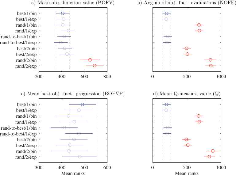
As shown in Table 3, all DE variants are able to produce results close to or better than the best known objective function value f*. Moreover, eight out of ten DE variants have a success ratio close to 1. Variants rand/2/{bin, exp} are the only ones with a lower success ratio, scoring 0.6 and 0.52 respectively. According to column
In terms of efficiency, the variants best/1/{bin, exp} and rand-to-best/1/{bin, exp}have the lowest average number of objective function evaluations (Table 3, column
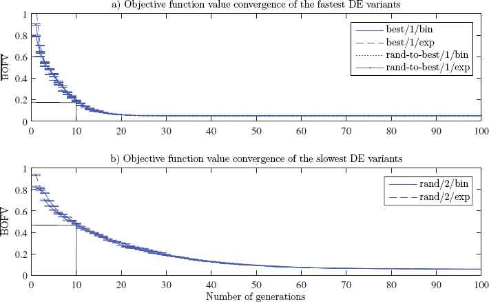
For this optimization instance, variants best/1/{bin, exp} and rand-to-best/1/{bin, exp} needed an average of 40 generations or 794 objective function evaluations to reach the best known objective value, whereas 95 generations were needed for rand/2/{bin, exp}. When considering both efficacy and efficiency measures, variants best/1/{bin, exp}and rand-to-best/1/{bin, exp} are equally applicable. Fig. 6 summarizes the classification of the DE variants in terms of efficacy and efficiency. For the structured controller design problem instance, variants best/1/{bin, exp} and rand-to-best/1/{bin, exp} are both efficacious and efficient. Variants rand/1/{bin, exp} and best/2/{bin, exp} are efficacious, and variants rand/2/{bin, exp} are neither efficacious nor efficient.
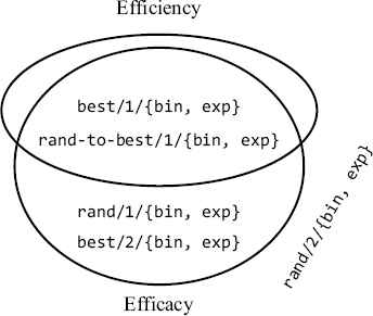
DE variants classification for the structured controller design problem instance.
7. Conclusion
In this paper, ten DE variants were used to design a low-order and fixed structure controller. Their performances were compared in terms of efficacy and efficiency measures. Bootstrap estimation was used to estimate success ratio, mean best objective function values, empirical probability density, average number of objective function evaluations, and mean objective function value progression.
Inference using nonparametric multiple comparison tests indicated that variants best/1/{bin, exp}and rand-to-best/1/{bin, exp} have the best success ratios, mean objective function accuracies, and average number of objective function evaluations. The probability density estimations of their outputs also revealed their ability to reach the best known objective function values with high probability. Variants rand/1/{bin, exp} and best/2/{bin, exp}produced the same mean objective function accuracies, but have a higher-than-average number of objective evaluations. Finally, variants rand/2/{bin,exp} showed lower objective function accuracies and higher requirements for the number of objective evaluations.
This work has shown that the proposed solution method is effective for low-order fixed structure controller design. Higher order controllers should become cost-effective in the near future, as new reconfigurable embedded hardware promises more data throughput and an increase in computing power. Thus, further research is needed to ascertain the impact on BMI formulation and DE optimization for high-order controller design. More work is also needed to overcome the difficulties of DE parameter tuning. As with other evolutionary algorithms, DEs are sensitive to control parameter changes and must be tuned. One way to alleviate the problem is to apply adaptive control mechanisms. The parameters to be adapted can be encoded directly in each individual and undergo mutation and crossover operations.19 Good control parameter values will bring forth better individuals and propagate them to future generations. Another adaptive approach is to obtain feedback information from the search and update control parameters accordingly. Lastly, an interesting technique is to compute a population diversity measure and use it to adapt F and CR at each generation.20
References
Cite this article
TY  - JOUR
AU  - Tony Wong
AU  - Pascal Bigras
AU  - Vincent Duchaîne
AU  - Jean-Philippe Roberge
PY  - 2016
DA  - 2016/09/01
TI  - Empirical Comparison of Differential Evolution Variants for Industrial Controller Design
JO  - International Journal of Computational Intelligence Systems
SP  - 957
EP  - 970
VL  - 9
IS  - 5
SN  - 1875-6883
UR  - https://doi.org/10.1080/18756891.2016.1237193
DO  - 10.1080/18756891.2016.1237193
ID  - Wong2016
ER  -