
Interactive TOPSIS Based Group Decision Making Methodology Using Z-Numbers
- DOI
- 10.1080/18756891.2016.1150003How to use a DOI?
- Keywords
- Type-1 fuzzy number; interval type-2 fuzzy number; z-number; multi-criteria decision making; TOPSIS; stock selection; reliability of information
- Abstract
The ability in providing result that is consistent with actual ranking remains the major concern in group decision making environment. The main aim of this paper is to introduce a novel modification of TOPSIS method to facilitate multi criteria decision making problems based on the concept of Z-numbers called Z-TOPSIS. The proposed method is adequate and intuitive in giving meaningful structure for formalizing information of a decision making problem, as it takes into account the decision makers’ reliability. This study also provides bridge with some established knowledge in fuzzy sets to certain extend as to strengthen the concept of ranking alternatives using Z – numbers. To ensure practicality and effectiveness of proposed method, stock selection problem is studied. The ranking based on proposed method is validated comparatively using spearman rho rank correlation. Based on the analysis, the proposed method outperforms the established TOPSIS methods in term of ranking performance.
- Copyright
- © 2016. the authors. Co-published by Atlantis Press and Taylor & Francis
- Open Access
- This is an open access article under the CC BY-NC license (http://creativecommons.org/licences/by-nc/4.0/).
1. Introduction
There has an increasing interest in group decision making technique and a considerable amount of study has published on it. In about forty years since it is introduced, over 70 Multi Criteria Decision Making (MCDM) techniques has developed for facilitating decision making practice [1]. MCDM is a practical tool for selection and ranking of a number of alternatives, its applications are numerous[2]–[5]. Amongst the techniques available, the frequently used are Simple Additive Weighting (SAW)[6], Analytical Hierarchy Process (AHP) [7], ELimination and Choice Expressing REality(ELECTRE)[8], and Technique for Order Preference by Similarity to Ideal Solution (TOPSIS)[9].
SAW method is based on the weighted average. An assessment score is considered for all alternatives by multiply the scaled importance given to the alternative of that element with the weights of relative importance directly assigned by decision maker. However, SAW uses only for maximizing assessment criteria, while minimizing assessment criteria should be transformed into the maximizing ones by the respective formulas prior to their relevance [10]. While for AHP, it is based on the decision maker assigning a relative value of weight for all of the criteria by pair-wise comparison. The shortcoming is that the exhaustive pair-wise comparison is tiresome and time consuming when there are a lot of alternatives to considered. On the other hand, ELECTRE which is introduce by [11], is categorised into three namely Choice problematic, ranking problematic and sorting problematic. For ranking problematic, ELECTRE II, ELECTRE III and ELECTRE IV are used. They are concerned with the ranking of all the activities belonging to a specified set of activities from the greatest to the worst. A major problem with the ELECTRE methods is they use similar threshold values but provide different ranking towards alternatives. Therefore, the aforementioned techniques have limitations from one to another.
In contrary, TOPSIS which is introduced in 1981[12], it is a helpful technique in dealing with MCDM problems in real life. It chooses the best alternative in a problem by taking the alternative that has the shortest distance from the positive ideal solution and the farthest from the negative ideal solution. It helps Decision Makers (DMs) solve the problem through analysis, comparisons and rankings of the alternatives. TOPSIS has deemed one of the major decision making techniques. In recent years, TOPSIS has been effectively applied to the areas of human resources management [13], transportation [5], product design [14], manufacturing [15], water management [16], quality control [4], military [2], tourism [17] and location analysis [18]. In addition, the concept of TOPSIS has also been connected to multi-objective decision making and group decision making. The high flexibility of this concept is able to accommodate further extension to make better choices in various situations.
According to [19] and [20], TOPSIS has the following three advantages: (i) a sound logic that represents the rationale of individual choice; (ii) a scalar value that record for both the best and worst alternatives concurrently; and (iii) a straightforward computation algorithm that can be easily programmed into a spreadsheet. These advantages make TOPSIS a popular MCDM technique as compared with other related techniques such as AHP and ELECTRE[21]. In fact, TOPSIS is a value-based process that compares each alternative directly depending on information in the evaluation matrices and weights [5]. Thus, TOPSIS is chosen as the main body of expansion in this study.
In 2000, TOPSIS methodology was introduced for the first time in fuzzy environment which believed can provide additional flexibility to represent the uncertainty comparison to non-fuzzy TOPSIS by [22]. After a decade, researcher has established TOPSIS methodology using interval type 2 fuzzy set, which supposed can offer further degree of freedom to represent the uncertainty and the fuzziness of the real world comparison to type 1 version of TOPSIS[23]. Nevertheless, the reliability of the decision information and the experience of the expert are not well taken into consideration in decision process. Therefore the problems arise how confident the decision makers are about their decision. According to [24], the issue of reliability of information is very important in decision making environment as this is extensively discussed in [25].The concept of Z-numbers captures the fuzziness of information better than type- 1 and interval type-2 fuzzy set. They provide an additional feature which is the reliability of decision makers in representing the fuzziness of the decision makers’ preference. Hence, in this methodology, the concept of Z-numbers introduced by [25] has been used to propose a novel modification of TOPSIS called Z-TOPSIS. This modification is more effective and intuitively significant for formalising the information structure of decision making problem.
The paper is organized as follows. In the next section, theoretical preliminaries for TOPSIS are given. Section 3 focuses on the proposed TOPSIS method, with various combinations in an algorithm-by-algorithm fashion. Afterwards, the case study on stock selection problem is conducted to illustrate the usefulness of proposed method. For the analysis purposes these results are compared with returns on investment as benchmarking and validated comparatively using Spearman rho rank correlation. In the final section, conclusions are drawn.
2. Basic Terms and Definitions
In the following, we briefly review some basic definitions of fuzzy sets. These basic definitions and notations are used throughout the paper unless stated otherwise.
Definition 1 [22]:
Fuzzy set
A fuzzy set A is defined on a universe X may be given as:
Where μA(x): X →[0,1] is the membership function A. The membership value μA(x) describes the degree of belongingness of x ∈ X in A.
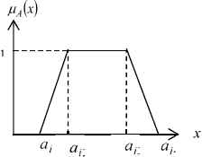
Throughout this paper, type-1 fuzzy number, interval type-2 fuzzy number and Z-number are presented in the form of trapezoidal fuzzy number. It is easy to deal with because it is piece wise linear. On the other hand, the good coverage of trapezoidal fuzzy number is a good compromise between efficiency and effectiveness.
Definition 2 [22]:
Type-1 Fuzzy Number
A trapezoidal fuzzy numbers can be represented by the following membership function given by
Definition 2[26]:
Interval Type-2 Fuzzy Set
A type-2 fuzzy set à in the universe of discourse X is represented by a type-2 membership function μà follows:
Where JX denotes an interval in [0, 1]. A type-2 fuzzy set à can also be represented as:
Definition 3 [23]:
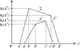
Interval Type-2 Fuzzy Number
A trapezoidal interval type-2 fuzzy set à can be represented by
Type-1 Fuzzy Number
Interval type-2 Fuzzy Number
Definition 4 [27]:
Z-number
Z-number is an ordered pair of type-1 fuzzy numbers denoted as
The concept of a Z-numbers,
(Very good, Likely), (Good, Unlikely)
Z – number,
3. Proposed Method
A systematic approach to extend the TOPSIS using Z-number is proposed in this section. Step 1 is the extension of non-fuzzy TOPSIS, where the concept of Z-number is introduced into the formulation. Z – number enhance the capability of both type – 1 and type – 2 fuzzy numbers by taking into account the reliability of the numbers used[25].This concept is very suitable for solving group decision-making problem in fuzzy environment.
In this paper, the importance weights of various criteria and the ratings of qualitative criteria are considered as linguistic variables. These linguistic variables can be expressed in positive trapezoidal fuzzy numbers as Tables 1, 2 and 3.
| Linguistic Variables | Trapezoidal Fuzzy Number |
|---|---|
| Very Low (VL) | (0.00, 0.00, 0.00, 0.10) |
| Low (L) | (0.00, 0.10, 0.10, 0.25) |
| Medium Low (ML) | (0.15, 0.30, 0.30, 0.45) |
| Medium (M) | (0.35, 0.50, 0.50, 0.65) |
| Medium High (MH) | (0.55, 0.70,0.70, 0.85) |
| High (H) | (0.80, 0.90, 0.90, 1.00) |
| Very High (VH) | (0.90, 1.00, 1.00, 1.00) |
Linguistic Variables for the Importance Weight of Each Criterion
| Linguistic Variables | Trapezoidal Fuzzy Number |
|---|---|
| Very Poor (VP) | (0, 0, 0, 1) |
| Poor (P) | (0, 1, 1, 3) |
| Medium Poor (MP) | (1, 3, 3, 5) |
| Fair (F) | (3, 5, 5, 7) |
| Medium Good (MG) | (5, 7, 7, 9) |
| Good (G) | (7, 9, 9, 10) |
| Very Good (VG) | (9, 10, 10, 10) |
Linguistic Variables for the Ratings of all alternative
| Linguistic Variables | Trapezoidal Fuzzy Number |
|---|---|
| Strongly Unlikely (SU) | (0.00, 0.00, 0.00, 0.10) |
| Unlikely (U) | (0.00, 0.10, 0.10, 0.25) |
| Somewhat Unlikely (SWU) | (0.15, 0.30, 0.30, 0.45) |
| Neutral (N) | (0.35, 0.50, 0.50, 0.65) |
| Somewhat Likely (SWL) | (0.55, 0.70, 0.70, 0.85) |
| Likely (L) | (0.80, 0.90, 0.90, 1.00) |
| Strongly Likely (SL) | (0.90, 1.00, 1.00, 1.00) |
Linguistic Variables for the Expert’s Reliability
In [22], it is suggested that the decision makers use the linguistic variables in Table 1, 2 to evaluate the importance of the criteria and the ratings of alternatives with respect to various criteria. In addition to this, Table 3 is proposed here, which is implementing the Z-TOPSIS formulation to deal on decision makers’ reliability. The importance of criteria, the rating of alternatives and the reliability of decision makers can be written in the form
The following algorithm is conducted to get the ranking of alternatives, whereby Step 1 is purely from [24] but it make use the linguistics variable for expert’s reliability from Table 3 for the component B in Z-number, follows by Step 2–7 are adopted from [22].
Z-TOPSIS ALGORITHM
Step 1: Used the Information from Table 3 to Derive Component B, and Then Convert Z-Number to Type-1 Fuzzy Number
Assume a Z-number,
Step 2: Construct Decision Matrix
Assume that a decision group has K persons, and then the importance of the criteria and the rating of alternatives with respect to each criterion can be calculated as in Eq. (4).
Multi criteria decision making problem can easily expressed in matrix format as shown in Eq. (5).
Step 3: Construct Normalized Fuzzy Decision Matrix,
The technique mentioned on top of is to preserve the property that the ranges of normalized fuzzy numbers belong to [0,1].
Step 4: Construct the Weighted Normalized Fuzzy Decision Matrix,
Considering the different importance of each criterion, we can construct the weighted normalized fuzzy decision matrix as shown in Eq. (7)
Step 5: Find Fuzzy Positive-Ideal Solution, A* and Fuzzy Negative-Ideal Solution, A−
Based on the weighted normalized fuzzy decision matrix, the elements
Step 6: Find Distance of Each Alternative from A* and A−
The distance of each alternative from A*and A− can be currently calculated as shown in Eq. (9).
Step 7: Find Closeness Coefficient, CCi
A closeness coefficient is defined to determine the ranking order of all alternatives once the
4. Application to a Stock Selection Problem
In this case study the evaluation is done by three decision makers. These financial experts including finance lecturer, fund manager and PhD finance student. They evaluated 25 Securities listed on Main Board in Bursa Malaysia at 30 November 2007 and then make investment recommendations according to financial ratio considered. The stocks are Green Packet Bhd(S1), Malaysian Pacific Industries(S2), AIC Corp Bhd(S3), MesiniagaBhd(S4), HeiTechPaduBhd(S5), D&O Ventures Bhd(S6), Pentamaster Corp Bhd(S7), ENG Teknologi HldgsBhd(S8), Patimas Computers Bhd(S9), Metronic Global Bhd(S10), Globetronics Technology Bhd(S11), Unisem M Bhd(S12), GHL Systems Bhd(S13), Kobay Technology Bhd(S14), AliranIhsan Resources Bhd(S15), PuncakNiaga Holding Bhd(S16), Ranhill Utilities Bhd(S17), Digi.Com Bhd(S18), Time dotComBhd(S19), LingkaranTransKotaHldg(S20), YTL Power International Bhd(S21), BIMB Holdings Bhd(S22), Pan Malaysia Holdings Bhd(S23), Syarikat Takaful Malaysia(S24), Kuchai Development Bhd(S25).
The most importance ratio considered in investment is Market Value of Firm (C1) defined as Market value of firm-to-earnings before amortization, interest and taxes ratio. This ratio is one of the most frequently used financial indicators and the lower this ratio is better [28]. Return on Equity (C2) used to examine how much the company earns on the investment of its shareholders. Portfolio managers examine this ratio very carefully and used it when deciding whether to buy or sell. The higher the ratio is better. Dept/equity ratio (C3), this ratio belongs to long term solvency ratios that are intended to address the firm’s long run ability to meet its obligations. So, it is assume by DMs that the lower the ratio the better[29]. Current ratio (C4) is one of the ways to measure liquidity of company. It explains the ability of a business to meet its current obligations when fall due. Higher the ratio is better[30]. Market value/net sales (C5) is market value ratios of particular interest to the investor are earnings per common share, the price-to-earnings ratio, market value-to book value ratio, earning-to-price ratio. The lower the ratio is the better[31]. Price/earnings ratio (C6) measure the ratio of market price of each share of common stock to the earnings per share, the lower this ratio is better. In the case study, the alternative of decision makers to be rank and to be weighted according to the above mention ratios are 25 stocks listed in Bursa Malaysia.
In this study, Microsoft Excel is used to calculate all the calculation involved in the evaluating the ranking of stocks and the weight of each criterion. The processes of evaluating the ranking and weight of each stock are as follow the proposed methods. The DMs use the linguistic weighting variable in Table 1 to assess the importance of the criteria ,and make use information in Table 3 to measure the DMs reliability when assess the criteria then we represent it in the z-number form Z = (A, B)as Table 4 below:
| DM1 | DM2 | DM3 | ||||
|---|---|---|---|---|---|---|
| Criteria | A | B | A | B | A | B |
| (C1) | VH | L | H | L | VH | SL |
| (C2) | MH | SWL | MH | SL | MH | L |
| (C3) | H | SL | M | SWL | H | SL |
| (C4) | M | L | ML | L | MH | L |
| (C5) | H | SL | MH | SL | ML | SWL |
| (C6) | ML | L | ML | L | ML | L |
Importance of the criteria and the DMs reliability
Afterward, the DMs use the linguistic rating variable in Table 2 to evaluate the rating of stock with respect to each criterion and use information in Table 3 to cooperate DMs reliability in evaluating the stock performance with respect to each criterion as presented in Table 5, 6 and 7 (see Annexes ).
All linguistic terms can be express as trapezoidal fuzzy number as shown in Table 1, 2 and 3. The Z-TOPSIS Algorithm introduced in Section 3 is now illustrated for the case study of stock selection problem.
Step 1: Used the Information from Table 3 to Derive Component B, and Then Convert Z-Number to Type-1 Fuzzy Number
In this step, using Eq. (1)–(3), the important of criteria C1 from Table 4 is used to illustrate the procedure of proposed approach. Assume Decision Maker 1 (DM1) give his opinion as follows:
à = (0.9,1.0,1.0,1.0;1)
The DMs knowledge can be expressed to Z-number as:
At first, we should convert DMs reliability into crisp number
Second, add the weight of reliability to the constraint.
Third, convert the weighted Z-number to Type-1 fuzzy number according to proposed approach.
Repeat the same procedure for all DM’s judgments. By considering the decision makers reliability, the importance of the criteria and the rating of all alternative were obtained in the Table 8.
| DM1 | DM2 | DM3 | |
|---|---|---|---|
| C1 | (0.8538 0.9487 0.9487 0.9487) | (0.7589 0.8538 0.8538 0.9487) | (0.8849 0.9832 0.9832 0.9832) |
| C2 | (0.4602 0.5857 0.5857 0.7112) | (0.5408 0.6882 0.6882 0.8357) | (0.5218 0.6641 0.6641 0.8064) |
| C3 | (0.7866 0.8849 0.8849 0.9832) | (0.2928 0.4183 0.4183 0.5438) | (0.7866 0.8849 0.8849 0.9832) |
| C4 | (0.3320 0.4743 0.4743 0.6166) | (0.1423 0.2846 0.2846 0.4269) | (0.5218 0.6641 0.6641 0.8064) |
| C5 | (0.7866 0.8849 0.8849 0.9832) | (0.5408 0.6882 0.6882 0.8357) | (0.1255 0.2510 0.2510 0.3765) |
| C6 | (0.1423 0.2846 0.2846 0.4269) | (0.1423 0.2846 0.2846 0.4269) | (0.1423 0.2846 0.2846 0.4269) |
Z-weight matrix for each criterion
Step 2: Construct Z- Average Decision Matrix,
Considering Eq. (4), the fuzzy decision matrix and the fuzzy weight of each criterion is constructed.
In this case, the rating of S1 and weight respect to C1 is calculated as below.
Therefore the average rating for S1 is
In order to define Z-average weight matrix using Eq. (4)
Therefore the average weighting for S1 is
Step 3: Construct a Normalized Z- Decision Matrix (
Thus, the normalized Z-decision matrix is as in Table 10 (see Annexes ).
Step 4: Construct the weight normalize Z-decision making matrix (
To construct fuzzy weighted normalized fuzzy decision matrix, Let
Step 5: The Fuzzy Positive-Ideal Solution A* and Fuzzy Negative-Ideal Solution A−
The fuzzy positive ideal solution and fuzzy negative ideal solution are defined based on Eq. (8).
Step 6: Distance of Each Alternative from Ã* And Ã−
The distance between weights normalized rating
Next, using Eq. (16) for S1
| Stock | D+ | D− |
|---|---|---|
| S1 | 3.68 | 3.43 |
| S2 | 4.98 | 2.13 |
| S3 | 5.84 | 1.27 |
| S4 | 4.66 | 2.48 |
| S5 | 5.49 | 1.65 |
| S6 | 5.20 | 1.92 |
| S7 | 4.30 | 2.81 |
| S8 | 4.88 | 2.25 |
| S9 | 5.91 | 1.16 |
| S10 | 4.96 | 2.19 |
| S11 | 4.72 | 2.40 |
| S12 | 4.51 | 2.64 |
| S13 | 5.11 | 2.02 |
| S14 | 5.04 | 2.08 |
| S15 | 4.91 | 2.24 |
| S16 | 4.78 | 2.35 |
| S17 | 5.16 | 1.95 |
| S18 | 5.00 | 2.11 |
| S19 | 5.43 | 1.67 |
| S20 | 4.54 | 2.55 |
| S21 | 4.82 | 2.32 |
| S22 | 5.41 | 1.73 |
| S23 | 4.33 | 2.80 |
| S24 | 5.49 | 1.66 |
| S25 | 4.46 | 2.70 |
Distance each alternative from Ã* and Ã−
Step 7: The Closeness Coefficient of Each Criterion, CCi
Based on the distance of alternative in Table 11, the closeness coefficient for each alternative are derived using Eq. (10). For example, the closeness coefficient for S1 is calculated using Eq. (10) as follows:
The closeness coefficient and the ranking of 25 stocks based on proposed method is shown in Table 12.
| RANK | STOCK | CC |
|---|---|---|
| 1 | Green Packet Bhd(S1), | 0.48 |
| 2 | Pentamaster Corp Bhd(S7), | 0.40 |
| 3 | Pan Malaysia Holdings Bhd(S23), | 0.39 |
| 4 | Kuchai Development BHD (S25). | 0.38 |
| 5 | Unisem M Bhd(S12), | 0.37 |
| 6 | Lingkaran TransKota Hldg (S20), | 0.36 |
| 7 | Mesiniaga Bhd(S4), | 0.35 |
| 8 | Globetronics Technology BHD(S11), | 0.34 |
| 9 | Puncak Niaga Holding BHD (S16), | 0.33 |
| 10 | YTL Power International Bhd(S21), | 0.32 |
| 11 | ENG Teknologi Hldgs BHD (S8), | 0.32 |
| 12 | Aliran Ihsan Resources Bhd (S15), | 0.31 |
| 13 | Metronic Global Bhd(S10), | 0.31 |
| 14 | Malaysian Pacific Industries(S2), | 0.30 |
| 15 | Digi.Com BHD (S18), | 0.30 |
| 16 | Kobay Technology BHD(S14), | 0.29 |
| 17 | GHL Systems Bhd(S13), | 0.28 |
| 18 | Ranhill Utilities Bhd(S17), | 0.27 |
| 19 | D&O Ventures Bhd(S6), | 0.27 |
| 20 | BIMB Holdings Bhd(S22), | 0.24 |
| 21 | Time dotCom Bhd(S19), | 0.24 |
| 22 | Syarikat Takaful Malaysia (S24), | 0.23 |
| 23 | HeiTech Padu Bhd(S5), | 0.23 |
| 24 | AIC Corp BHD (S3), | 0.18 |
| 25 | Patimas Computers Bhd (S9), | 0.16 |
Ranking of 25 stocks based on Z-TOPSIS
5. Discussion of Results
The ranking produced by Z-TOPSIS (see Table 12) is compared with the type-1 TOPSIS method and interval type-2 TOPSIS method as shown in Table 13 and 14, where DMs reliability is not considered. The returns on investment for a month trading period have been used for validation purposes. Investment is dynamic process, since longer the investment period, the greater the risk. It depends on the return on investment. If the percentage is higher, investors very quickly sell their share. So, for this study one month investment is preferable.
| TYPE 1- TOPSIS METHOD | ||
|---|---|---|
| RANK | STOCK | CC |
| 1 | Green Packet Bhd(S1), | 0.6565 |
| 2 | Kuchai Development BHD (S25). | 0.5361 |
| 3 | Pentamaster Corp Bhd(S7), | 0.5341 |
| 4 | Puncak Niaga Holding BHD (S16), | 0.5183 |
| 5 | Unisem M Bhd(S12), | 0.5072 |
| 6 | Globetronics Technology BHD(S11), | 0.5044 |
| 7 | Pan Malaysia Holdings Bhd(S23), | 0.5043 |
| 8 | Mesiniaga Bhd(S4), | 0.4976 |
| 9 | Lingkaran TransKota Hldg (S20), | 0.4821 |
| 10 | ENG Teknologi Hldgs BHD (S8), | 0.4812 |
| 11 | Aliran Ihsan Resources Bhd (S15), | 0.4535 |
| 12 | Malaysian Pacific Industries(S2), | 0.4495 |
| 13 | Metronic Global Bhd(S10), | 0.4489 |
| 14 | YTL Power International Bhd(S21), | 0.4483 |
| 15 | BIMB Holdings Bhd(S22), | 0.4436 |
| 16 | GHL Systems Bhd(S13), | 0.4401 |
| 17 | Digi.Com BHD (S18), | 0.4348 |
| 18 | Kobay Technology BHD(S14), | 0.4256 |
| 19 | D&O Ventures Bhd(S6), | 0.4088 |
| 20 | Ranhill Utilities Bhd(S17), | 0.4001 |
| 21 | HeiTech Padu Bhd(S5), | 0.3853 |
| 22 | Syarikat Takaful Malaysia (S24), | 0.3665 |
| 23 | Time dotCom Bhd(S19), | 0.3640 |
| 24 | Patimas Computers Bhd (S9), | 0.2756 |
| 25 | AIC Corp BHD (S3), | 0.2559 |
Ranking based on type 1 TOPSIS
| TYPE 2- TOPSIS METHOD | ||
|---|---|---|
| RANK | STOCK | CC |
| 1 | Green Packet Bhd(S1), | 0.94 |
| 2 | Pentamaster Corp Bhd(S7), | 0.77 |
| 3 | Pan Malaysia Holdings Bhd(S23), | 0.69 |
| 4 | Unisem M Bhd(S12), | 0.68 |
| 5 | Lingkaran TransKota Hldg (S20), | 0.66 |
| 6 | Kuchai Development BHD (S25). | 0.63 |
| 7 | Mesiniaga Bhd(S4), | 0.61 |
| 8 | ENG Teknologi Hldgs BHD (S8), | 0.60 |
| 9 | Puncak Niaga Holding BHD (S16), | 0.59 |
| 10 | Globetronics Technology BHD(S11), | 0.56 |
| 11 | YTL Power International Bhd(S21), | 0.56 |
| 12 | Metronic Global Bhd(S10), | 0.54 |
| 13 | Kobay Technology BHD(S14), | 0.53 |
| 14 | Digi.Com BHD (S18), | 0.53 |
| 15 | Aliran Ihsan Resources Bhd (S15), | 0.51 |
| 16 | Malaysian Pacific Industries(S2), | 0.50 |
| 17 | Ranhill Utilities Bhd(S17), | 0.48 |
| 18 | GHL Systems Bhd(S13), | 0.47 |
| 19 | D&O Ventures Bhd(S6), | 0.46 |
| 20 | BIMB Holdings Bhd(S22), | 0.44 |
| 21 | HeiTech Padu Bhd(S5), | 0.39 |
| 22 | Syarikat Takaful Malaysia (S24), | 0.37 |
| 23 | Time dotCom Bhd(S19), | 0.37 |
| 24 | AIC Corp BHD (S3), | 0.35 |
| 25 | Patimas Computers Bhd (S9), | 0.34 |
Ranking based on interval type 2 TOPSIS
In the stock market, a price change or return in investment is the difference in trading prices from one period to the next or the difference between the daily opening and closing prices of a share of stock. For example, let's say Company Malaysian Pacific Industries (S2) shares opened at MYR8.60 and closed at MYR9.30. The price change is MYR0.7 or percentage of return is MYR0.7/MYR8.60 x 100 = 8.14% as shown in Table 15.
| Ranking | Stock | Returns (%) |
|---|---|---|
| 1 | AIC Corp BHD (S3), | 25.98 |
| 2 | Green Packet Bhd(S1), | 12.45 |
| 3 | AliranIhsan Resources Bhd (S15), | 11.21 |
| 4 | Malaysian Pacific Industries(S2), | 8.14 |
| 5 | PuncakNiaga Holding BHD (S16), | 6.38 |
| 6 | Pan Malaysia Holdings Bhd(S23), | 5.56 |
| 7 | YTL Power International Bhd(S21), | 3.05 |
| 8 | Globetronics Technology BHD(S11), | 2.27 |
| 9 | Kobay Technology BHD(S14), | 1.45 |
| 10 | Kuchai Development BHD (S25). | 0.95 |
| 11 | D&O Ventures Bhd(S6), | 0.00 |
| 12 | Digi.Com BHD (S18), | −0.40 |
| 13 | Unisem M Bhd(S12), | −0.60 |
| 14 | Syarikat Takaful Malaysia (S24), | −0.63 |
| 15 | Time dotComBhd(S19), | −0.69 |
| 16 | LingkaranTransKotaHldg (S20), | −1.02 |
| 17 | Pentamaster Corp Bhd(S7), | −1.54 |
| 18 | Ranhill Utilities Bhd(S17), | −2.04 |
| 19 | HeiTechPaduBhd(S5), | −2.20 |
| 20 | BIMB Holdings Bhd(S22), | −2.88 |
| 21 | MesiniagaBhd(S4), | −4.35 |
| 22 | Metronic Global Bhd(S10), | −6.25 |
| 23 | Patimas Computers Bhd (S9), | −9.09 |
| 24 | ENG Teknologi Hldgs BHD (S8), | −9.86 |
| 25 | GHL Systems Bhd(S13), | −10.87 |
Ranking of 25 stocks based on returns on investment
In the real stock market, the greater the positive price change/returns, the more desirable the stock. Likewise, the greater the negative price change/returns the less desirable the stock. The statistical method, spearman rho correlation, is used in this study to identify and test the strength of a relationship between ranking based on TOPSIS methods and ranking based on returns on investment. At the same time, its measure the efficiency in terms of methods based on rankings performance as shown in Table 16.
| No. | Stock | Actual | T1 (EM) | IT2 (EM) | Z (PM) | T1 (EM) | IT2 (EM) | Z-TOPSIS (PM) | |||
|---|---|---|---|---|---|---|---|---|---|---|---|
| ∂i | ∂i | ∂i | |||||||||
| 1 | S1 | 2 | 1 | 1 | 1 | 1 | 1 | 1 | 1 | 1 | 1 |
| 2 | S2 | 4 | 12 | 16 | 14 | −8 | 64 | −12 | 144 | −10 | 100 |
| 3 | S3 | 1 | 25 | 24 | 24 | −24 | 576 | −23 | 529 | −23 | 529 |
| 4 | S4 | 21 | 8 | 7 | 7 | 13 | 169 | 14 | 196 | 14 | 196 |
| 5 | S5 | 19 | 21 | 21 | 23 | −2 | 4 | −2 | 4 | −4 | 16 |
| 6 | S6 | 11 | 19 | 19 | 19 | −8 | 64 | −8 | 64 | −8 | 64 |
| 7 | S7 | 17 | 3 | 2 | 2 | 14 | 196 | 15 | 225 | 15 | 225 |
| 8 | S8 | 24 | 10 | 8 | 11 | 14 | 196 | 16 | 256 | 13 | 169 |
| 9 | S9 | 23 | 24 | 25 | 25 | −1 | 1 | −2 | 4 | −2 | 4 |
| 10 | S10 | 22 | 13 | 12 | 13 | 9 | 81 | 10 | 100 | 9 | 81 |
| 11 | S11 | 8 | 6 | 10 | 8 | 2 | 4 | −2 | 4 | 0 | 0 |
| 12 | S12 | 13 | 5 | 4 | 5 | 8 | 64 | 9 | 81 | 8 | 64 |
| 13 | S13 | 25 | 16 | 18 | 17 | 9 | 81 | 7 | 49 | 8 | 64 |
| 14 | S14 | 9 | 18 | 13 | 16 | −9 | 81 | −4 | 16 | −7 | 49 |
| 15 | S15 | 3 | 11 | 15 | 12 | −8 | 64 | −12 | 144 | −9 | 81 |
| 16 | S16 | 5 | 4 | 9 | 9 | 1 | 1 | −4 | 16 | −4 | 16 |
| 17 | S17 | 18 | 20 | 17 | 18 | −2 | 4 | 1 | 1 | 0 | 0 |
| 18 | S18 | 12 | 17 | 14 | 15 | −5 | 25 | −2 | 4 | −3 | 9 |
| 19 | S19 | 15 | 23 | 23 | 21 | −8 | 64 | −8 | 64 | −6 | 36 |
| 20 | S20 | 16 | 9 | 5 | 6 | 7 | 49 | 11 | 121 | 10 | 100 |
| 21 | S21 | 7 | 14 | 11 | 10 | −7 | 49 | −4 | 16 | −3 | 9 |
| 22 | S22 | 20 | 15 | 20 | 20 | 5 | 25 | 0 | 0 | 0 | 0 |
| 23 | S23 | 6 | 7 | 3 | 3 | −1 | 1 | 3 | 9 | 3 | 9 |
| 24 | S24 | 14 | 22 | 22 | 22 | −8 | 64 | −8 | 64 | −8 | 64 |
| 25 | S25 | 10 | 2 | 6 | 4 | 8 | 64 | 4 | 16 | 6 | 36 |
| 0 | 1992 | 0 | 2128 | 0 | 1922 | ||||||
| Rho coefficient (ρ) | 0.234 | 0.182 | 0.261 | ||||||||
| Methods Ranking according performance | 2 | 3 | 1 | ||||||||
TOPSIS Ranking Performance Based on Spearman Rho Correlation for Established Methods (EM) and Proposed Method (PM)
For the validation purposes, the authors consider the rankings based on existing non rule based approach and returns on investment. These rankings are compared descriptively using Spearman rho correlation.
The Advantages of this correlation method are its easy algebraic structure and intuitively simple interpretation. Besides this, the method is less sensitive to bias due to the effect of outliers and can be used to reduce the weight of outliers, i.e. large distances get treated as a one-rank difference.
In general, the coefficient of rho (ρ) measures the strength of association between two ranked variables. The formula used to calculate Spearman’s Rank is shown in Eq. (11)
Based on the analysis in Table 16, it is observed that the proposed method, Z-TOPSIS, outperform the existing non rule based approach in term of ranking performance.
6. Summary
This paper introduces a novel Z-TOPSIS method-extending the capability of the new concept of Z number within multi-criteria decision making analysis particularly TOPSIS. Proposed method takes into account the decision maker reliability very well. Compared to existing TOPSIS methods based on type 1 and interval type 2, Z- TOPSIS can efficiently represent uncertain information. Based on analysis of results, Z-TOPSIS produces the most significant rho coefficient comparison to others established TOPSIS methods. It seems to be more effective and intuitively significant for formalizing information structure of a decision making problem. Proposed method also has more powerful to describe the knowledge of human being and will be widely used in uncertainty information process. Furthermore, this study also provides bridge with some established knowledge in fuzzy sets to certain extend as to strengthen the concept of ranking alternatives using Z – numbers.
Annexes
| DECISION MAKER 1 | ||||||||||||
|---|---|---|---|---|---|---|---|---|---|---|---|---|
| STOCK | CRITERIA | |||||||||||
| C1 | C2 | C3 | C4 | C5 | C6 | |||||||
| A | B | A | B | A | B | A | B | A | B | A | B | |
| S1 | VG | N | VG | N | G | N | VG | L | G | L | G | SWL |
| S2 | VP | SWL | VG | SWL | F | L | P | SWL | G | L | G | SL |
| S3 | VP | L | VP | SL | G | SL | P | L | VP | L | F | SL |
| S4 | F | L | MP | N | F | N | G | L | MP | SWL | G | SL |
| S5 | P | SWL | P | L | F | SWL | F | N | P | SL | F | L |
| S6 | VP | N | G | SL | F | SL | F | SWL | VP | L | F | SWL |
| S7 | VG | L | F | SWL | F | L | F | SL | G | SL | F | N |
| S8 | F | N | F | N | F | N | F | L | P | N | VG | SL |
| S9 | VP | SL | VP | SL | F | SWL | P | L | VP | SWL | F | L |
| S10 | F | N | G | N | F | SL | F | SL | P | SL | F | SL |
| S11 | P | SWL | G | L | F | N | F | L | P | N | G | SL |
| S12 | G | N | G | SL | F | L | F | SWL | P | L | F | SWL |
| S13 | P | L | G | SL | F | N | VG | L | P | N | F | L |
| S14 | F | N | P | SWL | F | SWL | G | L | P | SWL | VG | N |
| S15 | P | SL | F | N | F | SL | G | SWL | P | SL | F | SL |
| S16 | F | N | VG | SL | F | L | G | SL | P | L | F | SWL |
| S17 | P | N | VG | SL | VP | N | F | N | P | N | P | N |
| S18 | P | SWL | VG | L | G | SWL | F | L | P | SWL | VG | L |
| S19 | VP | SL | VP | N | F | SL | G | SL | F | SL | F | SL |
| S20 | VG | SL | G | SL | F | N | F | SWL | G | L | VG | N |
| S21 | P | L | VG | SWL | G | L | F | L | P | N | F | SWL |
| S22 | F | SL | F | N | F | N | P | SL | F | SL | P | SL |
| S23 | VG | SWL | P | SL | F | SWL | G | L | F | SWL | VG | L |
| S24 | VP | SL | G | L | P | SL | F | L | F | SL | F | N |
| S25 | VG | L | F | SL | F | L | G | SL | G | L | G | SWL |
Rating of 25 stocks by DM1 for all criteria
| DECISION MAKER 2 | ||||||||||||
|---|---|---|---|---|---|---|---|---|---|---|---|---|
| STOCK | CRITERIA | |||||||||||
| C1 | C2 | C3 | C4 | C5 | C6 | |||||||
| A | B | A | B | A | B | A | B | A | B | A | B | |
| S1 | VG | SL | VG | L | F | SL | MG | SWL | MG | SL | F | SWL |
| S2 | P | L | VG | SWL | G | L | F | L | MG | SL | F | SL |
| S3 | P | SWL | VP | SL | G | SWL | F | SL | P | SWL | F | SWL |
| S4 | MP | L | F | SWL | VG | SWL | G | SWL | P | L | F | L |
| S5 | P | N | F | L | VG | SL | G | SWL | VP | SWL | MG | SL |
| S6 | P | SWL | MG | SWL | VG | L | G | SWL | VP | SWL | MG | L |
| S7 | VG | L | MG | SL | F | SWL | F | SL | G | N | G | N |
| S8 | G | L | MG | L | G | SWL | G | N | P | L | P | SL |
| S9 | P | N | VP | SWL | VG | B | F | SWL | F | L | F | N |
| S10 | F | L | G | SL | F | L | G | L | P | SL | G | SWL |
| S11 | F | SL | G | SWL | VG | SL | VG | N | F | SL | F | L |
| S12 | MG | SWL | G | L | G | L | F | SWL | F | SWL | MG | SL |
| S13 | P | L | G | SL | VG | SWL | G | SL | VP | L | VG | SWL |
| S14 | G | L | F | SWL | VG | SL | G | SL | P | SWL | P | SL |
| S15 | MG | SL | G | L | G | SL | VG | L | F | SL | G | L |
| S16 | F | SWL | VG | SWL | P | N | G | N | F | L | G | SWL |
| S17 | F | SL | VG | L | VP | L | G | SWL | F | SWL | G | SL |
| S18 | F | L | VG | SL | G | SWL | F | SL | VP | L | F | SL |
| S19 | P | SL | P | SWL | VG | SL | G | SWL | G | SWL | F | SWL |
| S20 | VP | SWL | G | L | P | SL | G | L | G | N | F | L |
| S21 | G | SL | G | L | G | SL | G | L | P | SL | MG | SL |
| S22 | P | SL | P | SWL | F | SWL | F | SWL | F | SWL | MP | SWL |
| S23 | VG | SWL | F | SL | MG | L | G | SL | G | L | P | L |
| S24 | P | SL | MG | SL | VP | SL | G | SL | VP | SWL | F | SL |
| S25 | F | L | P | SWL | F | SL | VG | L | MG | SL | G | SL |
Rating of 25 stocks by DM2 for all criteria
| DECISION MAKER 3 | ||||||||||||
|---|---|---|---|---|---|---|---|---|---|---|---|---|
| STOCK | CRITERIA | |||||||||||
| C1 | C2 | C3 | C4 | C5 | C6 | |||||||
| A | B | A | B | A | B | A | B | A | B | A | B | |
| S1 | G | SWL | VG | SWL | VG | L | VG | SL | G | L | G | SL |
| S2 | VP | L | VG | L | P | N | VP | L | G | N | G | SWL |
| S3 | VP | N | VP | L | G | SL | P | N | P | SL | P | L |
| S4 | G | SL | G | SL | G | SWL | G | SWL | P | SWL | G | N |
| S5 | P | SWL | P | SWL | G | SL | P | SWL | P | L | G | SL |
| S6 | VP | SL | VG | SL | G | SL | P | SWL | P | SL | MP | L |
| S7 | G | N | VG | N | G | N | P | N | G | SL | P | SWL |
| S8 | F | SL | G | L | G | SL | P | L | P | SL | P | L |
| S9 | VP | SWL | VP | SL | VG | SL | P | SL | VP | SWL | VP | N |
| S10 | F | L | VG | SL | P | SL | P | SWL | P | N | VG | SL |
| S11 | P | SL | VG | SWL | G | SWL | G | SL | P | L | G | SWL |
| S12 | G | SL | VG | L | F | L | P | N | P | N | G | L |
| S13 | P | SWL | G | SL | MP | N | MP | L | VP | SL | VG | L |
| S14 | G | SL | P | SL | MP | SL | MP | SWL | VP | L | P | L |
| S15 | F | SL | P | L | P | L | MG | SL | P | L | MG | N |
| S16 | G | SL | F | SL | F | L | MP | SL | P | SWL | MG | L |
| S17 | G | L | G | SL | VP | SL | P | L | P | SL | G | SWL |
| S18 | P | SWL | VG | N | G | SL | VP | N | VP | N | P | N |
| S19 | VP | N | VP | L | VP | SWL | P | L | G | SL | F | L |
| S20 | G | SL | P | SWL | G | L | P | N | G | SWL | P | SWL |
| S21 | MP | SL | G | SL | P | N | P | SWL | P | SL | F | SL |
| S22 | F | L | F | SL | F | SL | P | SL | F | L | P | SL |
| S23 | G | SWL | P | SWL | G | SWL | G | SL | G | SWL | P | SWL |
| S24 | VP | SL | VG | SL | P | SL | MG | L | VP | SL | G | N |
| S25 | F | SL | F | L | F | L | F | L | F | SL | F | L |
Rating of 25 stocks by DM3 for all criteria
| WEIGHT | C1 | C2 | C3 | C4 | C5 | C6 |
|---|---|---|---|---|---|---|
|
|
||||||
| (0.83 0.93 0.93 0.96) | (0.51 0.65 0.65 0.78) | (0.62 0.73 0.73 0.84) | (0.33 0.47 0.47 0.62) | (0.48 0.61 0.61 0.73) | (0.14 0.28 0.28 0.43) | |
| STOCK | C1 | C2 | C3 | C4 | C5 | C6 |
| S1 | (7.02 8.14 8.14 8.42) | (7.48 8.31 8.31 8.31) | (5.48 6.92 6.92 7.81) | (7.19 8.39 8.39 8.95) | (6.07 7.99 7.99 9.27) | (5.08 6.85 6.85 8.02) |
| S2 | (0.00 0.32 0.32 1.54) | (7.87 8.74 8.74 8.74) | (3.16 4.66 4.66 6.08) | (0.95 1.86 1.86 3.37) | (5.50 7.26 7.26 8.47) | (5.23 7.10 7.10 8.36) |
| S3 | (0.00 0.28 0.28 1.39) | (0.00 0.00 0.00 0.97) | (6.54 8.41 8.41 9.34) | (0.98 2.19 2.19 3.95) | (0.00 0.61 0.61 2.14) | (1.82 3.35 3.35 5.19) |
| S4 | (3.56 5.48 5.48 7.07) | (3.37 5.05 5.05 6.41) | (5.17 6.48 6.48 7.23) | (6.46 8.31 8.31 9.23) | (0.28 1.43 1.43 3.18) | (4.89 6.65 6.65 7.85) |
| S5 | (0.00 0.79 0.79 2.38) | (0.95 2.18 2.18 4.00) | (6.08 7.62 7.62 8.51) | (2.66 3.97 3.97 5.28) | (0.00 0.64 0.64 2.21) | (4.88 6.82 6.82 8.44) |
| S6 | (0.00 0.28 0.28 1.40) | (6.64 8.18 8.18 9.06) | (6.12 7.75 7.75 8.73) | (2.79 4.18 4.18 5.58) | (0.00 0.33 0.33 1.58) | (2.73 4.56 4.56 6.38) |
| S7 | (7.34 8.45 8.45 8.68) | (4.60 6.05 6.05 7.26) | (3.45 5.13 5.13 6.56) | (1.97 3.51 3.51 5.30) | (6.24 8.02 8.02 8.91) | (2.36 3.58 3.58 4.84) |
| S8 | (3.90 5.66 5.66 7.11) | (4.50 6.24 6.24 7.66) | (4.95 6.64 6.64 7.72) | (2.60 4.02 4.02 5.52) | (0.00 0.88 0.88 2.64) | (2.95 3.92 3.92 5.21) |
| S9 | (0.00 0.24 0.24 1.31) | (0.00 0.00 0.00 0.93) | (5.91 7.03 7.03 7.59) | (0.84 2.04 2.04 3.88) | (0.95 1.58 1.58 2.77) | (1.66 2.76 2.76 4.10) |
| S10 | (2.60 4.34 4.34 6.08) | (6.89 8.35 8.35 8.91) | (1.93 3.55 3.55 5.49) | (3.20 4.76 4.76 6.29) | (0.00 0.89 0.89 2.67) | (5.88 7.43 7.43 8.36) |
| S11 | (0.98 2.25 2.25 4.11) | (6.68 8.14 8.14 8.74) | (5.61 6.97 6.97 7.72) | (5.36 6.89 6.89 7.85) | (0.98 2.19 2.19 3.95) | (5.19 7.04 7.04 8.28) |
| S12 | (5.34 7.02 7.02 8.14) | (7.35 8.96 8.96 9.60) | (4.13 6.04 6.04 7.63) | (1.67 3.02 3.02 4.61) | (0.84 1.95 1.95 3.61) | (4.69 6.53 6.53 8.06) |
| S13 | (0.00 0.91 0.91 2.73) | (6.88 8.85 8.85 9.83) | (3.45 4.67 4.67 5.62) | (5.46 7.06 7.06 8.02) | (0.00 0.24 0.24 1.35) | (6.30 7.53 7.53 8.16) |
| S14 | (5.21 6.97 6.97 8.09) | (0.84 2.00 2.00 3.77) | (4.11 5.65 5.65 6.87) | (4.79 6.63 6.63 7.83) | (0.00 0.56 0.56 1.99) | (2.12 3.00 3.00 4.29) |
| S15 | (2.62 4.26 4.26 6.23) | (2.92 4.34 4.34 5.76) | (3.28 4.90 4.90 6.52) | (6.44 7.97 7.97 8.90) | (0.98 2.28 2.28 4.23) | (4.38 6.13 6.13 7.58) |
| S16 | (3.84 5.52 5.52 6.88) | (6.44 7.70 7.70 8.36) | (1.91 3.43 3.43 5.17) | (4.27 6.05 6.05 7.27) | (0.95 2.18 2.18 4.00) | (4.37 6.12 6.12 7.59) |
| S17 | (3.20 4.72 4.72 6.16) | (8.09 9.39 9.39 9.72) | (0.00 0.00 0.00 0.88) | (2.66 4.00 4.00 5.39) | (0.84 1.96 1.96 3.64) | (4.25 5.70 5.70 6.77) |
| S18 | (0.95 2.14 2.14 3.89) | (7.92 8.80 8.80 8.80) | (6.20 7.97 7.97 8.85) | (1.93 3.22 3.22 4.74) | (0.00 0.28 0.28 1.39) | (3.83 5.04 5.04 6.16) |
| S19 | (0.00 0.33 0.33 1.55) | (0.00 0.28 0.28 1.39) | (3.93 4.92 4.92 5.85) | (4.25 5.78 5.78 7.01) | (5.23 7.10 7.10 8.36) | (2.77 4.61 4.61 6.46) |
| S20 | (5.24 6.23 6.23 6.83) | (4.51 6.07 6.07 7.28) | (2.92 4.35 4.35 5.80) | (3.05 4.48 4.48 5.82) | (5.82 7.48 7.48 8.31) | (3.07 4.22 4.22 5.41) |
| S21 | (2.62 4.25 4.25 5.86 | (7.02 8.58 8.58 9.23 ) | (4.51 6.03 6.03 7.15) | (3.16 4.71 4.71 6.21) | (0.00 0.89 0.89 2.67) | (3.46 5.33 5.33 7.20) |
| S22 | (1.93 3.55 3.55 5.49 | (1.69 3.10 3.10 4.78 ) | (2.53 4.21 4.21 5.90) | (0.84 2.05 2.05 3.92) | (2.77 4.61 4.61 6.46) | (0.28 1.49 1.49 3.36) |
| S23 | (6.97 8.09 8.09 8.37 | (0.98 2.25 2.25 4.11 ) | (4.37 6.12 6.12 7.59) | (6.80 8.74 8.74 9.72) | (5.00 6.75 6.75 7.90) | (2.85 3.76 3.76 4.95) |
| S24 | (0.00 0.33 0.33 1.64 | (6.80 8.42 8.42 9.39 ) | (0.00 0.66 0.66 2.29) | (4.82 6.74 6.74 8.34) | (0.98 1.64 1.64 3.57) | (3.34 4.94 4.94 6.30) |
| S25 | (4.78 6.38 6.38 7.67 | (1.93 3.50 3.50 5.34 ) | (2.88 4.80 4.80 6.72) | (6.09 7.69 7.69 8.65) | (4.84 6.78 6.78 8.41) | (5.19 7.04 7.04 8.28) |
Z- decision matrix and Z-weight of each criterion
| STOCK | C1 | C2 | C3 | C4 | C5 | C6 |
|---|---|---|---|---|---|---|
| S1 | (0.59 0.7692 0.769 0.8226) | (0.386 0.545894 0.55 0.663) | (0.35 0.514 0.514 0.665) | (0.24 0.405 0.405 0.561) | (0.3 0.494 0.494 0.69) | (0.074 0.2 0.2 0.348) |
| S2 | (0.00 0.0299 0.03 0.1508) | (0.406 0.574269 0.57 0.697) | (0.2 0.346 0.346 0.518) | (0.03 0.09 0.09 0.211) | (0.27 0.449 0.449 0.63) | (0.076 0.21 0.21 0.363) |
| S3 | (0.00 0.0263 0.026 0.1356) | (0 0 0 0.078) | (0.41 0.624 0.624 0.795) | (0.03 0.106 0.106 0.248) | (0 0.038 0.038 0.159) | (0.026 0.1 0.1 0.226) |
| S4 | (0.30 0.5175 0.518 0.6907) | (0.174 0.331881 0.33 0.511) | (0.33 0.481 0.481 0.615) | (0.22 0.401 0.401 0.579) | (0.01 0.089 0.089 0.237) | (0.071 0.19 0.19 0.341) |
| S5 | (0.00 0.0749 0.075 0.2325) | (0.049 0.142992 0.14 0.319) | (0.38 0.565 0.565 0.724) | (0.09 0.191 0.191 0.331) | (0 0.04 0.04 0.165) | (0.071 0.2 0.2 0.366) |
| S6 | (0.00 0.0263 0.026 0.1367) | (0.343 0.537399 0.54 0.723) | (0.39 0.575 0.575 0.743) | (0.09 0.202 0.202 0.35) | (0 0.02 0.02 0.117) | (0.04 0.13 0.13 0.277) |
| S7 | (0.62 0.7977 0.798 0.8479) | (0.237 0.397224 0.4 0.579) | (0.22 0.38 0.38 0.559) | (0.07 0.169 0.169 0.332) | (0.31 0.496 0.496 0.663) | (0.034 0.1 0.1 0.21) |
| S8 | (0.33 0.5349 0.535 0.694) | (0.232 0.409883 0.41 0.611) | (0.31 0.492 0.492 0.657) | (0.09 0.194 0.194 0.346) | (0 0.054 0.054 0.196) | (0.043 0.11 0.11 0.226) |
| S9 | (0.00 0.0223 0.022 0.1283) | (0 0 0 0.075) | (0.37 0.521 0.521 0.646) | (0.03 0.098 0.098 0.244) | (0.05 0.098 0.098 0.206) | (0.024 0.08 0.08 0.178) |
| S10 | (0.22 0.41 0.41 0.5935) | (0.356 0.548511 0.55 0.711) | (0.12 0.263 0.263 0.467) | (0.11 0.23 0.23 0.395) | (0 0.055 0.055 0.199) | (0.085 0.21 0.21 0.363) |
| S11 | (0.08 0.2121 0.212 0.4018) | (0.345 0.535167 0.54 0.697) | (0.35 0.517 0.517 0.657) | (0.18 0.332 0.332 0.492) | (0.05 0.135 0.135 0.294) | (0.075 0.2 0.2 0.36) |
| S12 | (0.45 0.6633 0.663 0.7954) | (0.38 0.588579 0.59 0.766) | (0.26 0.448 0.448 0.649) | (0.06 0.146 0.146 0.289) | (0.04 0.12 0.12 0.269) | (0.068 0.19 0.19 0.35) |
| S13 | (0.00 0.0861 0.086 0.267) | (0.355 0.581392 0.58 0.784) | (0.22 0.347 0.347 0.478) | (0.18 0.341 0.341 0.503) | (0 0.015 0.015 0.101) | (0.091 0.22 0.22 0.355) |
| S14 | (0.44 0.6587 0.659 0.79) | (0.043 0.13148 0.13 0.301) | (0.26 0.42 0.42 0.585) | (0.16 0.32 0.32 0.491) | (0 0.034 0.034 0.148) | (0.031 0.09 0.09 0.186) |
| S15 | (0.22 0.4024 0.402 0.6081) | (0.151 0.285215 0.29 0.46) | (0.21 0.364 0.364 0.555) | (0.22 0.384 0.384 0.558) | (0.05 0.141 0.141 0.315) | (0.063 0.18 0.18 0.329) |
| S16 | (0.32 0.5216 0.522 0.6719) | (0.333 0.50624 0.51 0.667) | (0.12 0.254 0.254 0.44) | (0.14 0.292 0.292 0.456) | (0.05 0.135 0.135 0.298) | (0.063 0.18 0.18 0.329) |
| S17 | (0.27 0.4458 0.446 0.6019) | (0.418 0.616908 0.62 0.775) | (0 0 0 0.075) | (0.09 0.193 0.193 0.338) | (0.04 0.121 0.121 0.271) | (0.061 0.16 0.16 0.294) |
| S18 | (0.08 0.202 0.202 0.3796) | (0.409 0.57798 0.58 0.702) | (0.39 0.591 0.591 0.754) | (0.07 0.155 0.155 0.298) | (0 0.017 0.017 0.103) | (0.055 0.15 0.15 0.268) |
| S19 | (0.00 0.031 0.031 0.151) | (0 0.018324 0.02 0.111) | (0.25 0.365 0.365 0.498) | (0.14 0.279 0.279 0.44) | (0.26 0.439 0.439 0.622) | (0.04 0.13 0.13 0.28) |
| S20 | (0.44 0.5881 0.588 0.6674) | (0.233 0.399124 0.4 0.581) | (0.18 0.323 0.323 0.493) | (0.1 0.216 0.216 0.365) | (0.29 0.462 0.462 0.618) | (0.044 0.12 0.12 0.235) |
| S21 | (0.22 0.4013 0.401 0.5727) | (0.362 0.564044 0.56 0.736) | (0.29 0.447 0.447 0.608) | (0.11 0.227 0.227 0.39) | (0 0.055 0.055 0.199) | (0.05 0.15 0.15 0.312) |
| S22 | (0.16 0.335 0.335 0.5362) | (0.087 0.203425 0.2 0.381) | (0.16 0.312 0.312 0.502) | (0.03 0.099 0.099 0.246) | (0.14 0.285 0.285 0.481) | (0.004 0.04 0.04 0.146) |
| S23 | (0.59 0.7639 0.764 0.8171) | (0.051 0.147523 0.15 0.328 | (0.28 0.454 0.454 0.646) | (0.23 0.422 0.422 0.609) | (0.25 0.417 0.417 0.588) | (0.041 0.11 0.11 0.215) |
| S24 | (0.00 0.031 0.031 0.16) | (0.351 0.553064 0.55 0.749 | (0 0.049 0.049 0.195) | (0.16 0.325 0.325 0.523) | (0.05 0.101 0.101 0.266) | (0.048 0.14 0.14 0.274) |
| S25 | (0.40 0.6028 0.603 0.7491) | (0.1 0.22988 0.23 0.426 | (0.18 0.356 0.356 0.572) | (0.21 0.371 0.371 0.543) | (0.24 0.419 0.419 0.626) | (0.075 0.2 0.2 0.36) |
Z -weighted Normalized decision Matrix
References
Cite this article
TY  - JOUR
AU  - Abdul Malek Yaakob
AU  - Alexander Gegov
PY  - 2016
DA  - 2016/04/01
TI  - Interactive TOPSIS Based Group Decision Making Methodology Using Z-Numbers
JO  - International Journal of Computational Intelligence Systems
SP  - 311
EP  - 324
VL  - 9
IS  - 2
SN  - 1875-6883
UR  - https://doi.org/10.1080/18756891.2016.1150003
DO  - 10.1080/18756891.2016.1150003
ID  - Yaakob2016
ER  -