
Intelligent Decision Support System for Real-Time Water Demand Management
- DOI
- 10.1080/18756891.2016.1146533How to use a DOI?
- Keywords
- Water Demand Management; Decision Support System; Multi-agent Systems; Neural Networks
- Abstract
Environmental and demographic pressures have led to the current importance of Water Demand Management (WDM), where the concepts of efficiency and sustainability now play a key role. Water must be conveyed to where it is needed, in the right quantity, at the required pressure, and at the right time using the fewest resources. This paper shows how modern Artificial Intelligence (AI) techniques can be applied on this issue from a holistic perspective. More specifically, the multi-agent methodology has been used in order to design an Intelligent Decision Support System (IDSS) for real-time WDM. It determines the optimal pumping quantity from the storage reservoirs to the points-of-consumption in an hourly basis. This application integrates advanced forecasting techniques, such as Artificial Neural Networks (ANNs), and other components within the overall aim of minimizing WDM costs. In the tests we have performed, the system achieves a large reduction in these costs. Moreover, the multi-agent environment has demonstrated to propose an appropriate framework to tackle this issue.
- Copyright
- © 2016. the authors. Co-published by Atlantis Press and Taylor & Francis
- Open Access
- This is an open access article under the CC BY-NC license (http://creativecommons.org/licences/by-nc/4.0/).
1. Introduction
Water is considered to be the most important natural resource. This basic resource is essential for all kinds of social and economic activities, as well as for the life and the health of the mankind. From this perspective, it is easy to justify the great importance of water management. This fact has been accentuated in recent years, mainly since the Earth Summit held in Rio in 1992, due to pressures caused by population growth, urbanization and industrialization. That is, the scarcity of resources and the respect for the environment have drawn a new context that threatens both the quality and the availability of this resource.
For the aforementioned reasons, policies regarding water have undergone major changes over the last two decades. Accordingly, the concept of Water Demand Management (WDM) has significantly evolved1. Its current definition encompasses five main goals2: (1) reducing the quantity and quality of water required to accomplish a specific task; (2) adjusting the nature of the task so it can be accomplished with less or lower quality water; (3) reducing losses in movement from source through use to disposal; (4) shifting time of use to off-peak periods; and (5) increasing the system ability to operate during droughts.
In this context, the effectiveness of a WDM system heavily depends on demand forecasting. This is not only about minimizing the water used to meet demand, but accurate forecasts have associated other benefits, such as the reduction of energy consumption in water catchment, purification and distribution processes. This fact highlights the importance of water demand forecasting, which can be divided into:
- •
Very long-term forecasting (decades)3, which crucially determines the design of the water supply system, e.g. tanks capacities and pipes dimensions.
- •
Long-term forecasting (years)4, which allows managers to develop plans for managing water demand, as well as adjustments in the distribution system.
- •
Mid-term forecasting (months)5, used to adjust previous planning, through comparing actual and planned data, as well as to determine water price.
- •
Short-term forecasting (days)6, which involves the implementation of supply plans, by setting the necessary systems to that effect.
- •
Very short-term forecasting (hours)7, which results in water conveyance from tanks to points-of-consumption when requited, in the right quantity and pressure.
Therefore, with the passing of time, smaller time horizon forecasts are demanded in order to meet the requirements of this new context. Long-term forecasts are not enough to reach a suitable water management, but in the current circumstances reliable short-term forecasts are essential8. Thus, to meet efficiently the demand, forecasts must be continuously available with the aim of9:
- •
In terms of operation and energy efficiency, determining optimal regulation and pumping schemes to supply the predicted demand.
- •
In terms of quality, combining water sources in the most appropriate way to achieve a given standard in the supplied water.
- •
In terms of vulnerability, detecting network losses and failures through comparing actual and expected flows.
From this perspective, this article proposes the application of modern Artificial Intelligence (AI) techniques to WDM. With the aim of drawing up a holistic approach to this issue, we have developed an Intelligent Decision Support System (IDDS). That is, we seek the system overall solution rather than tackling the different sub-problems separately. This is the main contribution of the paper in comparison to the existing literature, which includes several works focused on different aspects of the WDM system –mainly water demand forecasting. Since we aim to consider the overall problem in its entirety, the WDM system has been designed as a set of different kind of agents with complex interrelations among them. This Multi-Agent System (MAS), whose core is based on advanced forecasting techniques such as Artificial Neural Networks (ANNs), determines the optimal adjustment of pumping stations.
This research has emerged from the interest of the Water Company of Gijón10, a municipality of 300,000 inhabitants in the north west of Spain, in these emerging management techniques. It should be highlighted that it is not a real application but it aims to show how AI techniques can be combined within a multi-agent framework in order to develop an IDDS for WDM.
This article is structured in five sections, including this introduction. Section 2 reviews the most relevant and recent literature on AI applications to WDM. Section 3 describes the MAS, with the different agents that form it and their purpose, and the structure and relationships between them. Section 4 presents and discusses the numerical results obtained after testing the system with water demand time series. Finally, section 5 concludes according to the stated objectives and defines future work lines.
2. Background: AI Applications for WDM
One of the great challenges in WDM is, undoubtedly, water demand forecasting. During the last decades of the 20th century, some statistical models were applied in this field. For example, Maidment and Miaou11 used ARIMA methodology12 to express daily water demand as a function of rainfall and air temperature in nine US cities. Some years later, An et al.13 included other climatic factors within ARIMA models to forecast water demand. Shvartser et al.14 integrated this methodology in a pattern recognition approach, explaining in detail the development of the model and evaluating it for an water supply system in Israel. Other studies15 used these statistical methods on similar issues, such as power demand forecast.
From the beginning of this century, AI has been incorporated in WDM, since it is a highly complex problem conditioned by the interaction of multiple variables and developed in uncertain environments. AI can be defined as the discipline that builds processes that, when run on a physical structure, produce results that respond to the perceived inputs based on the stored knowledge. These techniques were mainly used to forecast water demand. Lertpalangsunti et al.16 were pioneers and developed a forecasting system that used various classical AI tools. The study was conducted for the city of Regina (Canada) and achieved a great reduction in the forecasting error in comparison with statistical alternatives.
2.1. Machine Learning applied to Water Demand Forecasting
In AI, Machine Learning is a subfield geared towards the creation of programs that generalize behaviors from unstructured information supplied as examples. The literature contains many Machine Learning applications to water demand forecasting.
Jain and Ormsbee17 used ANNs to estimate the maximum weekly demand through information on some climatic factors (frequency and volume of rainfall and water temperature) and recent demand. Liu et al.18 used the same technique on Weinan City (China). Nasseri et al.19 developed a hybrid model of Genetic Algorithm and Kalman Filter for monthly water demand forecasting, with excellent results exclusively from previous demand data. Genetic Algorithms were also applied to other phenomena with similar characteristics20. Solomatine and Shrestha21 incorporated Fuzzy Logic to the forecasting, while Tabesh and Dini22 relied on it to predict water consumption in Tehran (Iran). The application of Support Vector Machines to the matter was studied by Msiza et al.23, who compared its results with ANNs in different scenarios. Recently, Ponte et al.24 developed an ANN-based system that significantly outperformed statistical techniques in the hourly forecasting and water demand. This system was used to tackle a classical problem of distribution networks, the Bullwhip Effect25, which is not relevant in long-term management but was shown to act as a source of inefficiencies in real-time WDM. Other Machine Learning techniques that have been applied to water demand forecasting are Random Forest26 and Multivariate Adaptive Regression Splines27.
2.2. MAS in WDM
Distributed AI, another branch of AI, is oriented to the study of the necessary techniques for knowledge distribution and coordination, as well as the interactions between system and environment. In this sense, the system is designed as set of intelligent agents. An agent can be defined as a computer system capable of carrying out flexible and autonomous actions that affect their environment according to certain design goals. This multi-agent methodology allows one to tackle WDM from a new approach by integrating different breeds of agents in a more complex system, where to combine forecasting techniques with other elements. This way, the system can be directed towards another objective of greater amplitude.
The literature contains some applications of MAS in WDM. Moss and Edmonds28 created an agent-based model, applied to the Thames basin, to analyze the effects on some social parameters on water demand. Athanasiadis et al.29 developed a MAS that simulated customers behavior to evaluate different pricing policies in Thessaloniki (Greece). Galán et al.30 integrated social, urban dynamics, geography, and consumption models under a multi-agent framework, where they simulated different water demand scenarios for Valladolid (Spain). Zechman31 used multi-agent modeling to evaluate different management strategies in water distribution systems. Giuliani and Castelletti32 evaluated the interest of cooperation in large water resource systems. Ni et al.33 first carried out a dynamic study of water quality based on a Q-Learning Algorithm, and subsequently34 developed a MAS aimed at dynamic water quality assessment. Recently, Karavas et al.35 designed an energy management MAS for the design and control of autonomous polygeneration microgrids.
2.3. Overview of the Bibliographic Analysis
After the literature review, we summarize our main assessments:
- (i)
The extensive literature brings evidence that AI is a suitable approach to address the WDM issue given its complexity and scale.
- (ii)
Authors have used these methodologies (e.g. ANNs) mainly for consumption forecasting since it is one of the basic pillars in WDM. Small prediction errors can be reached without generalized differences among the various methods. The consideration of additional variables (e.g. climatic factors) improves the prediction but the need for the immediate availability of these data is a major limitation in real-time forecasting.
- (iii)
Multi-agent methodology allows managers to study WDM from a broader perspective. It is possible to combine forecasting techniques with other elements (e.g. economic and social) to focus on goals of different nature (e.g. improve water quality or optimize transportation system).
Under these circumstances, this paper exhibits how AI techniques can be applied to WDM. Looking for the forecast that minimizes some error criterion can be understood as a partial solution for a larger identity problem. From a holistic approach, a MAS can be used in order to find the best overall solution. We have developed an IDSS aimed at optimizing real-time WDM, whose core are IA forecasting methods –recent demands are the only input, given the complexity of real-time availability of other data.
3. Description of the IDDS
In order to design the MAS, we have considered a simple structure of a water supply network. In the upper level, there are various catchment points –usually natural sources, such as wellsprings and marshes fed into by rivers and groundwater. In the lower level, the points-of-consumption represent the distributed water demand. Between both levels, the supply tanks (storage reservoirs) are intermediate echelons that receive the water from the natural sources through the adduction lines and send it to the points-of-consumption through the conduction lines. The treatment station and the pumping station are also key elements. Figure 1 displays an overview of this water supply network. Figure 2 summarizes the structure of the water supply network of Gijon, which will be used as a basis in the development of the system.
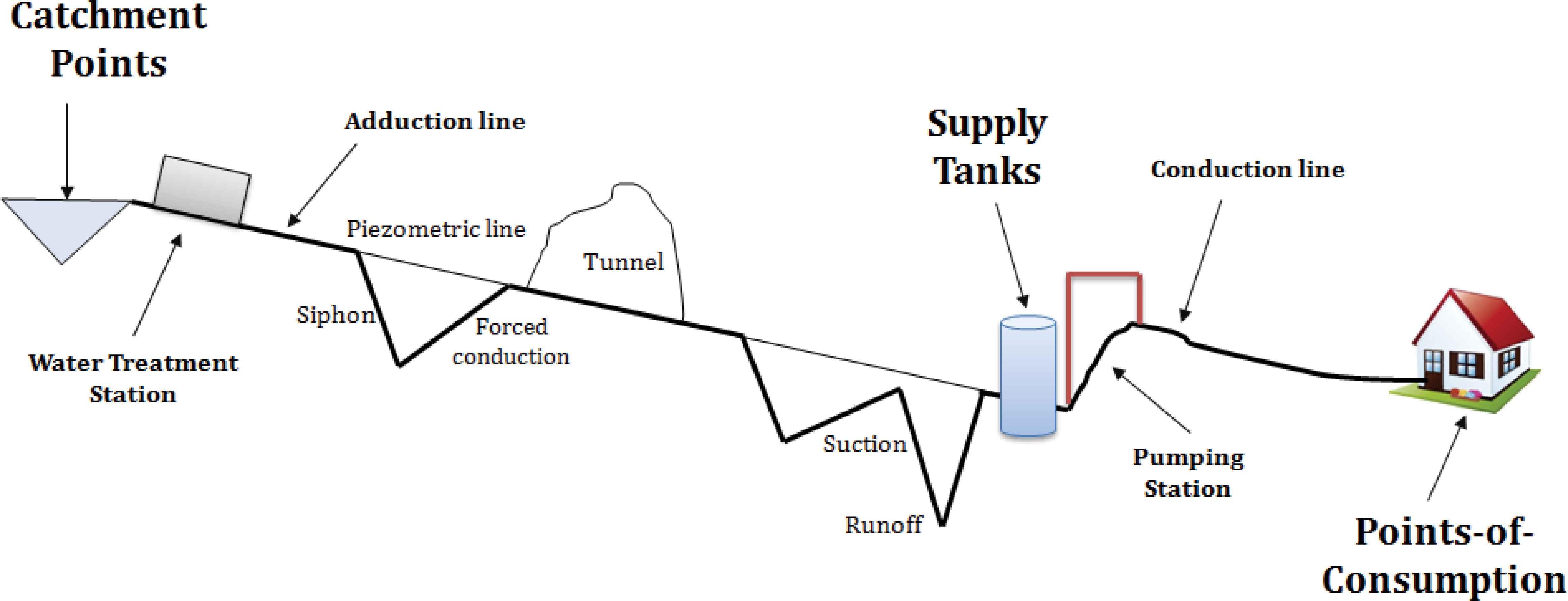
Overview of a water supply network.
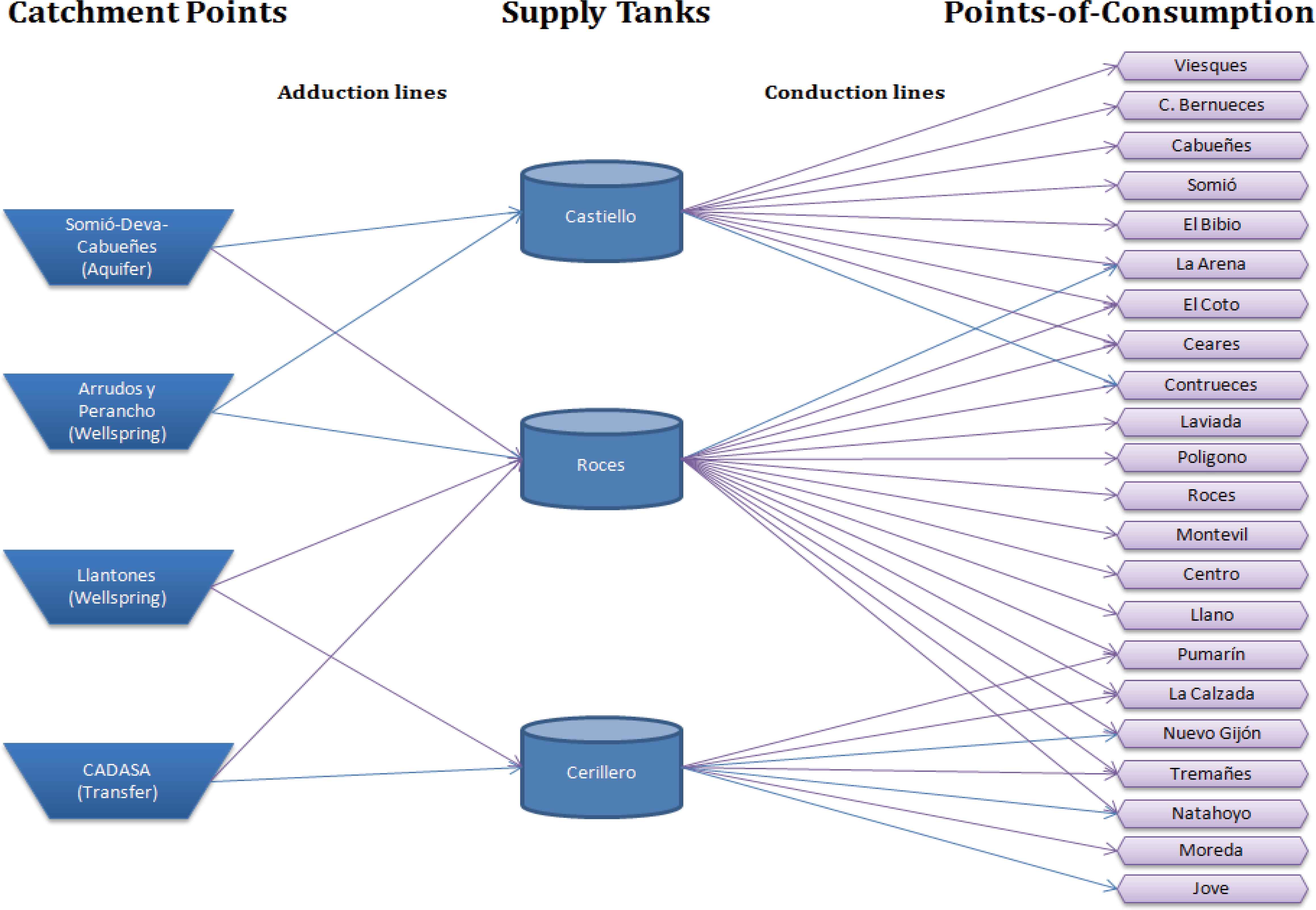
Basic structure of the water supply network of Gijón.
Figure 3 shows an outline of the structure of the IDSS that has been designed, with its agents and the relationships between them and with the outside. Input data are the real-time water demands (from the water demand measurement system in the points-of-consumption) and the supply tanks level (from the measurement system in the supply tanks). The output is the best adjustment of pumping systems, namely the optimum quantity of water to be pumped hourly from the supply tanks.
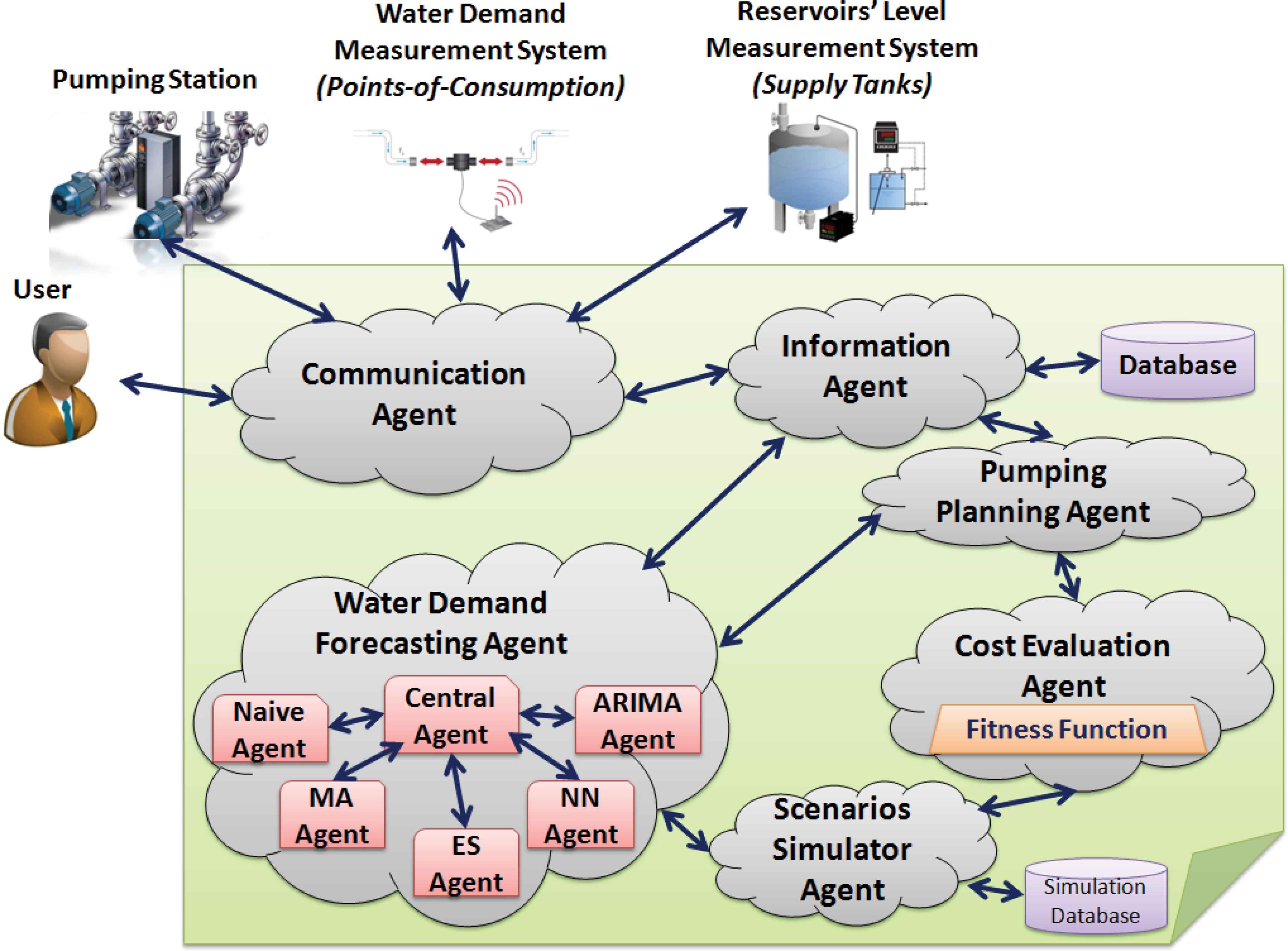
Outline of the IDSS that has been developed in this research work.
Six breeds of agents can be identified in the MAS. The bidirectional relationships between them are represented in Figure 3. Below, we explain in detail the function of the different breeds of agents.
- (i)
the Communication Agent,
- (ii)
the Information Agent,
- (iii)
the Water Demand Forecasting Agent,
- (iv)
the Scenarios Simulator Agent,
- (v)
the Cost Evaluation Agent,
- (vi)
the Pumping Planning Agent.
3.1. Communication Agent
The Communication Agent holds the interactions of the MAS with the outside. It operates in a quadruple way, as it communicates the MAS with:
- •
The water demand measurement system. Hence, hourly water demands are continuously stored in the database. This enables the development of reliable forecasts in real time.
- •
The reservoirs level measurement system. Thereby, the current level of the different supply tanks is continuously known and stored in the database, which has influence on the water to be pumped.
- •
The pumping stations, which operate according to the Pumping Planning Agent (it hourly determines the amount of water to be pumped).
- •
The user through an interface. The interface allows the user to introduce information that could alter the ordinary system operation (e.g. changes in the cost model or in the system’s constraints), as well as to see the most relevant information (e.g. consumption, forecasts, and costs).
3.2. Information Agent
The database associated to the Information Agent stores hourly data related to the WDM system, so that it is available for the other agents. In particular, it saves information on: (1) hourly water demand to date; (2) the most reliable demand forecasts to date; (3) water stored in supply tanks to date; and (4) hourly water pumped to date.
Thus, the main objective of the Information Agent is mediation between the database and the other agents, both storing data and responding to information requirements. Hence, the other agents do not see a database but another agent, and the MAS reaches the essential homogeneity.
3.3. Water Demand Forecasting Agent
The five forecasting agents are the real core of the MAS. Each one of them estimates the hourly water demand according to a predetermined method. Three simple forecasting methods (naive model, moving averages, and exponential smoothing), a complex statistical method (ARIMA models), and an AI-based tool (ANNs) are used. These calculate the forecasts using historical consumption stored in the database.
3.3.1 Naïve Agent
The Naive Agent performs the forecast using a naive model, which estimates the hourly demand (D^t) as the demand in the previous hour (Dt-1) adjusted by the increase (or decrease) in the demand in the same time interval of the previous week (Dt-168-Dt-169) by Eq. (1).
3.3.2 MA Agent
The MA Agent forecasts using a n-order moving average. It estimates the hourly demand (D^t) as the arithmetic average of the last n demands (Dt-i, i∈[1,n]). Previously, a 2nd-order differentiation (with the operator Δ) of the time series must be performed with the aim of eliminating trend and seasonality as the simple moving average method must not be applied for series with these features. The differentiation process is given by Eq. (2) and Eq. (3), while the forecast is based on Eq. (4) and requires undoing the differentiation process. The MA Agent calculates the forecast from n=1 (1 hour) to n=168 (1 week).
Among all forecasts, the MA Agent selects the optimal one according to the Mean Absolute Percentage Error (MAPE) criterion36, which is expressed by Eq. (5) where m is the time horizon.
3.3.3 ES Agent
The ES Agent forecasts according to a simple exponential smoothing with seasonality, i.e. a weighted average of the recent forecasts and the error in the same interval. Therefore, it estimates the hourly demand (D^t) as the sum of a level function associated with the last hour (Lt-1) and a seasonal function associated with the demand on the same day and hour of the week before (St-168) by Eq. (6). The level function depends on the linear smoothing coefficient (α) while the seasonal function depends on the seasonality coefficient (δ) as it can be seen in Eq. (7) and (8). Hence, the ES Agent evaluates different values of coefficients of linear smoothing and seasonality, seeking to minimize the MAPE.
3.3.4 ARIMA Agent
The ARIMA Agent estimates the hourly demand using an autoregressive integrated moving average model. These models can be synthesized according to [(p,d,q)(P,D,Q)n] where p (P) is the order of the autoregression, d (D) is the order of differentiation and q (Q) is the order of the moving average. The lowercase variables are not-seasonal components, while the uppercase ones are seasonal with periodicity n. These models consider that the future value of the differentiated variable (ΔdD^t) can be expressed as a function of past observations (Dt-i, i∈[1,n]) and a random error (εt-j, i∈[1,q]), by Eq. (9), where Δ is the differentiation operator, γ is the constant model, φi are the parameters associated with autoregression, and θj are the parameters associated with the moving average. It should be noted that it is also necessary to eliminate the differentiation.
The method of obtaining the statistical model [(p,d,q)(P,D,Q)n] associated with each time series is based on the sequential process of:
- (i)
identifying the possible model,
- (ii)
parameter estimation,
- (iii)
validation.
It should be highlighted that data from the last six weeks (1,008 hourly demands) are used in the forecasting. This process12 is repeated until both the model is verified through their autocorrelation functions and its forecasts are validated by a given error criterion. In our case, the ARIMA Agent seeks the model that best fits the input time series, using the following statistics for the comparison of the different proposed models:
- (i)
goodness-of -fit according to the MAPE criterion,
- (ii)
residual simple autocorrelation function,
- (iii)
residual partial autocorrelation function.
3.3.5 NN Agent
The NN Agent performs forecasting through ANNs with three levels: an input layer (predictor variables), a hidden layer, and one output neuron (variable to predict). The basic elements are the neurons in the hidden layer. Each one of them receives a number of inputs via interconnections and emits an output, which can be identified by three functions:
- (i)
a propagation or excitation function, which consists of the sum of each input by its interconnection weight,
- (ii)
an activation function, which modifies the former,
- (iii)
a transfer function, which is applied to the value returned by the above one and that limits the output.
Mathematically, the hourly demand forecast at each period (D^t) is expressed by Eq. (10), where yt represents the output (forecast), fouter represents de output layer, finner represents the input layer transfer function, wxy represents the weights and biases (i∈[1,17] refers to the input neurons and j∈[1,n] refers to the hidden neurons) and (z) represents the z-th layer.
Figure 4 outlines the designed ANN. We introduced 17 predictor variables (input neurons) in the NN Agent as the time series (see section IV) shows double periodicity: daily and weekly. The variables are: the day of the week (Day); the hour of the day (Hour); the four immediately preceding hourly demands (t-1 to t-4); the hourly demand of the day before at the same hour and the four immediately preceding demands (t-24 to t-28); the hourly demand of the previous week on the same day and the same hour and the four immediately preceding demands (t-168 to t-172); and an additional binary variable that differentiates holidays and working days (Holiday). The number of neurons in the hidden layer is a decision variable to optimize. The output neuron is related to the variable to predict: the hourly water demand. It should be clarified that we have looked for the best structure in terms of forecasting reliability, execution time (which is a significant limitation in a real-time system), and avoiding the common ‘overfitting’ problem (i.e. memorizing instead of learning).
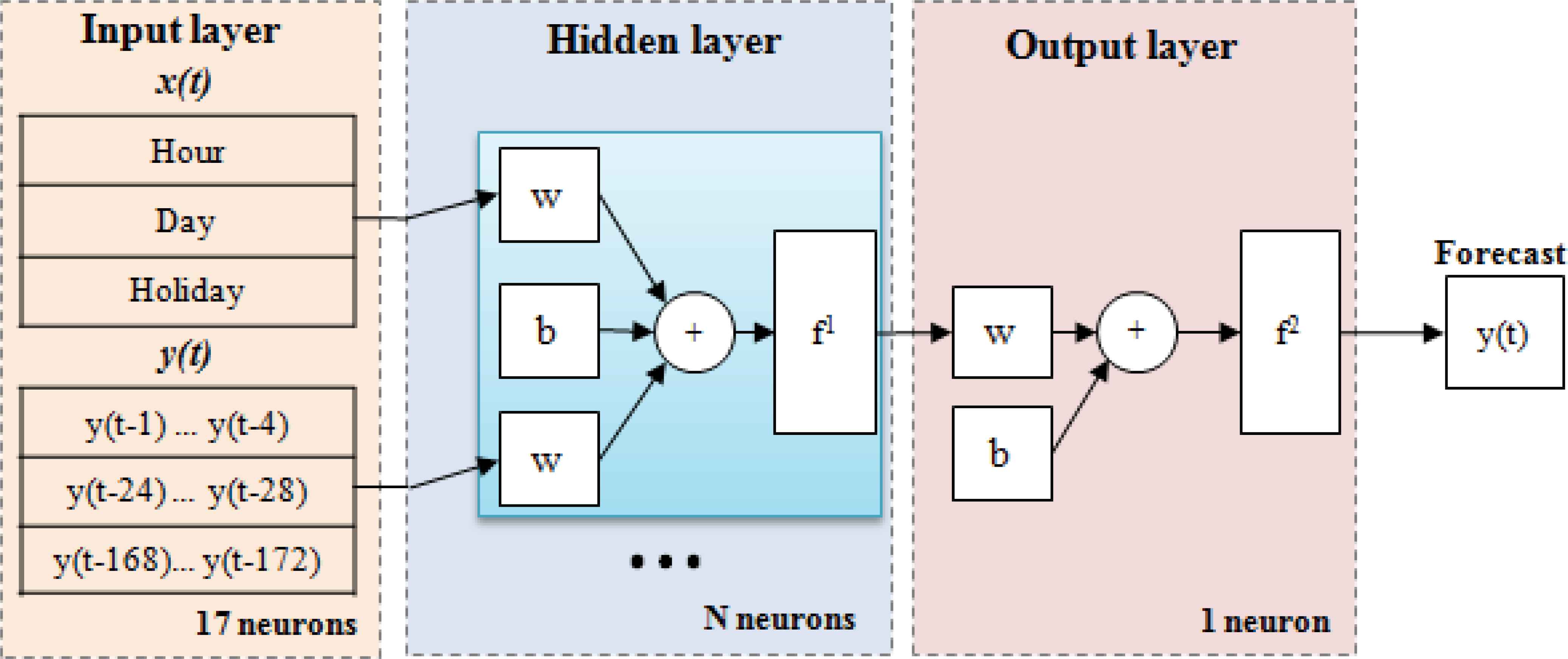
General outline of the ANN-based system.
The steps for developing the ANN-based system are similar to those detailed in Ref. 37, which can be considered as the preliminary step to this research work. This article forecasts hourly water demand comparing two different ANN architectures: multi-layer perceptron and radial basis functions, and concluded that the first structure tends to offer better performance. For this reason, a multi-layer perceptron has been used. The data available for each forecast, i.e. the last 6 weeks (1,008 hourly demands), were separated randomly into two groups. The 70% was oriented to the batch training of the network through the back-propagation algorithm. The remaining 30% has been used to validate the network. The following stopping criteria were defined:
- •
max number of steps without reducing error: 1000,
- •
max workout time: 1 minute.
- •
min relative change in training error: 0.0001,
- •
min relative change in error rate training: 0.001.
3.3.6 Central Agent
The optimal forecast selected hourly by each one of the five agents is sent to the Central Agent. These hourly demand forecasts are stored in the database through the Information Agent. Moreover, the Central Agent sends these forecasts to the Planning Pumping Agent. Therefore, the Central Agent only acts as interconnection between the Forecasting Agents and the other agents.
3.4. Scenarios Simulator Agent
In WDM systems, water pumping is performed at specific times whose frequency varies greatly from one city to another. The new context stresses the importance of continuous pumping in order to reduce operating costs. The Scenarios Simulator Agent uses information stored in the database to perform a simulation of the last 24 hours in different scenarios defined by the forecasts transmitted by the Central Agent. These will be studied by the Cost Evaluation Agent that seeks the one that minimizes WDM costs.
The assumptions that we have made in the development of this simulator are the following:
- •
fixed supply time: 1 hour (both, on the one hand, from natural sources to supply tanks and, on the other hand, from these to points-of-consumption),
- •
unconstrained catchment, storage and transportation systems,
- •
water is pumped to the supply tanks in order to store at the beginning of each hour the quantity that has been forecast,
- •
when there is risk of shortage, the pumping is carried out urgently at a higher cost,
- •
water cannot be returned to the previous echelon.
In order to determine the water stored at the beginning of each hour in Supply Tanks (IWt), this agent adds the water stored at the end of the last hour (FWt-1) and the water pumped during that time (WPt-1), by Eq. (11). The water stored at the end of each hour in Supply Tanks (FWt) is expressed as the difference between water stored at the beginning of this hour (IWt) and the hourly demand (Dt), except if this value is negative. In that case, the emergency water pumping (EWPt) would be carried out, and the water stored would be zero. It is expressed by Eq. (12) and (13). Finally, the water pumped in each period (WPt), a process that is supposed to be done at the end of it, is the difference between the demand forecast for the next period (D^t+1) and the final status of tank (FWt), if this value is greater than zero, according to Eq. (14).
The operational logic of the simulation system is illustrated in Figure 5. It should be noted that there are two main flows: the downstream water flow, from natural sources to points-of-consumptions and constrained by the lead time (supply time), and the upstream demand flow, in the opposite direction.
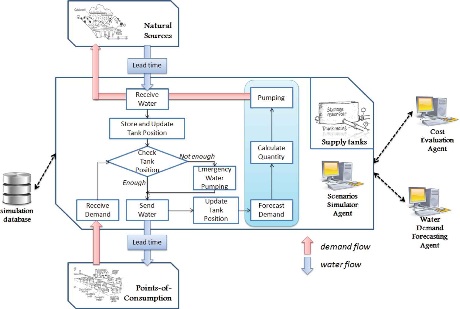
Overview of the simulation model, by means of a flow chart.
3.5. Cost Evaluation Agent
The Cost Evaluation Agent hourly decides which one of the five scenarios presented by the Scenarios Simulation Agent minimizes WDM costs and, therefore, it is optimal for managing the system at that time. In the simple structure previously defined and according to the stated assumptions, we consider that there is a cost associated with pumping, treatment and storage of water, which depends entirely on demand. That is to soy, water must be transported to the demand points, which involves some costs that are independent of the planning. Moreover, there are two cost overruns (both can be expressed as a ratio of a unit of currency to a unit of volume of water), which are inputs for the system:
- •
An additional cost associated with emergency water pumping (cewp), defined as the difference between the emergency water pumping cost and the scheduled water pumping cost.
- •
An additional cost related to excessive storage of water in Supply Tanks (cfw), in relation to tanks capacity and supply problems resulting from excessive storage of water, i.e. an opportunity cost.
Thus, the Cost Evaluation Agent determines in each scenario the WDM cost overrun (WMO), which arises from the errors in the forecast. It can be estimated as the sum of the cost overrun associated to the emergency water pumping (WMOewp) and the cost overrun associated to the excessive storage of water (WMOfw) throughout the simulation time interval (m). The first one is the product of emergency water pumped (EWPt) and its associated cost overrun (cewp). The second one is the product of the quantity of water stored at the end of each interval (FWt) and their additional costs associated storage (cfw). Hence, the fitness function to be minimized is expressed by Eq. (15) to (17).
3.6. Pumping Planning Agent
The Pumping Planning Agent uses the optimal scenario selected by the Cost Evaluation Agent to choose the forecast which must be used to adjust the pumping system. Hence, it determines the water to be pumped hourly by Eq. (14), but considering the position level of the supply tanks (instead of the simulation calculations) leading to real-time WDM. These data are stored in the database via the Information Agent, and they are carried to the Pumping Station through the Communication Agent.
4. Results and Discussion
In order to test the IDSS, twelve time series with 1,032 data (WD01 to WD12) have been used. Each one of them contains hourly water demands of 43 consecutive days in the city of Gijón (Spain). These time series have been created through simulation using the monthly water demand of this city, a distribution model of water demand along each week, and random parameters to introduce different sources of uncertainty. It should be clarified that the average hourly demand in the township in 2012 and 2013 was 2,455.44 m3/hour, while we have used the model that, according to Ref. 9, best fits the urban consumption in the city of Valencia (Spain).
Within each series, we have used 97.7 % of the data (1,008 hourly demands corresponding to 6 weeks) for training of forecasting methods and determining the optimal alternative for the pumping systems adjustment through simulation scenarios, while the remaining 2.3% (24 time demands, corresponding to 1 day) was used to test the system with the solution provided. From that point on, we have analyzed the reduction achieved in management costs.
The time series we have chosen span training and testing periods of very different nature. Table 1 contains the relevant information about the training period (first and last day) and testing period (day and hour of beginning and end). Note that in all cases the testing period begins when the training period ends. Six series have been chosen as working days (see [1]), which would be the usual case in the practical implementation of the system. Three series correspond to weekend days (see [2]). The remaining three are related to holidays (i.e. holidays or days around them, see [3]), since we aim to evaluate the effectiveness of the developed application in these special cases.
| Time series | Training period | Testing period | Features |
|---|---|---|---|
| WD01 | Jun 28, 2012 – Aug 9, 2012 | Thur 14 h - Frid 13 h | [1] |
| WD02 | Feb 8, 2013 – Feb 19, 2013 | Tues 03 h - Wedn 02 h | [1] |
| WD03 | Sep 28, 2012 – Nov 9, 2012 | Frid 11 h - Satu 10 h | [3] |
| WD04 | Feb 18, 2012 – Mar 30, 2012 | Satu 21 h - Sund 20 h | [2] |
| WD05 | Aug 15, 2012 – Sep 26, 2012 | Wedn 16 h - Thur 15 h | [1] |
| WD06 | Sep 12, 2011 – Oct 31, 2012 | Mond 09 h - Tues 08 h | [1] |
| WD07 | Nov 9, 2012 – Dec 22, 2012 | Sund 00 h - Sund 23 h | [2] |
| WD08 | Jan 4, 2012 - Feb 15, 2012 | Wedn 04 h - Thur 03 h | [1] |
| WD09 | Feb 23, 2013 – Apr 6, 2013 | Satu 13 h - Sund 12 h | [2] |
| WD10 | Apr 2, 2012 - May 14, 2012 | Mond 22 h - Tues 21 h | [1] |
| WD11 | May 15, 2012 - Jun 26, 2012 | Tuesd 16 h - Wedn 15 h | [3] |
| WD12 | Oct 24, 2012 – Dec 6, 2012 | Tues 06 h - Wedn 05 h | [3] |
It corresponds to a week after a holiday on Friday.
It corresponds to a week after a holiday on Tuesday.
Training and testing period for the time series.
The twelve time series show a similar structure. These hourly time series displays double seasonality and trend. On the one hand, there is a daily frequency (each 24 hours). There is a night sharp decrease from 19h until 02h, when demand stabilizes around a daily minimum until 06h. At that time, demand grows strongly until 11h, when it sets a first local maximum. From there, demand undergoes a slight decline to set a local minimum at 14h, and then it begins to increase until the establishment of a second local maximum at 19h. Note that the previously given hours are approximate and vary according to the season of the year. On the other hand, there is a weekly frequency, namely the structure is similar each 7 days (168 hours). During weekends, a significant decline in consumption can be observed –first on Saturdays, and even larger on Sundays, where the morning cycle is especially small compared to the afternoon one. In addition, these time series do not remain in a constant range, but they show a significant trend throughout the year, both in average and variance, which must be considered in the forecasting process. Figure 6, which has been included to illustrate the explanation, shows the training and testing periods for the time series WD03. Notice the decreasing trend from weeks 2 to 6, which seems to be reversed during the last week. Besides, the holidays in weeks 3 and 6, when demand drops considerably, greatly influence the forecast –especially the Friday of week 6, given the weekly frequency of the series, makes complicated the forecast.
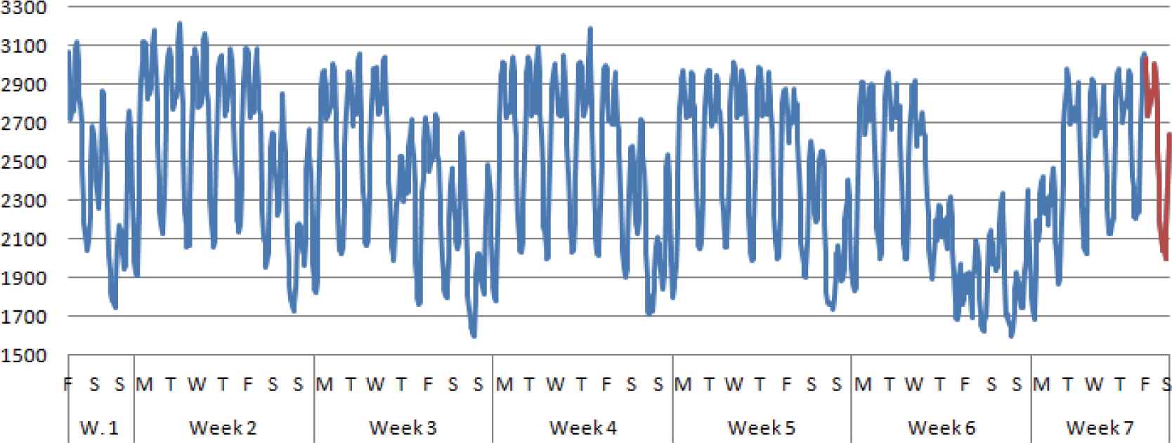
Training period and testing period for the time series WD03 (values in cubic meters).
4.1. Time Series Forecasting
The reduction in WDM costs is based on the accuracy of the system forecasts. Table 2 shows for each series the best result of the five forecasting agent. It contains the following information: the name of the time series (Time series); the agent that forecasts (Forecasting); the optimal features of the method that minimize the MAPE during the training period, i.e. the time horizon if it is a moving average, the linear smoothing and seasonality coefficient in the case of exponential smoothing, the ARIMA model that best fits the input data for the Box Jenkins methodology, and the optimal structure of the ANN through the neurons in each layer (Features); and the MAPE of the forecast calculated on the 24 testing data (MAPE). We have stood out in bold the agent which achieves a minimum error for each series.
| Time series | Forecasting | Features | MAPE |
|---|---|---|---|
| WD01 | Base Method | - | 1.11% |
| Naive Agent | - | 1.25% | |
| MA Agent | 5 | 2.81% | |
| ES Agent | α=0,8 ; δ=2,8·10-5 | 3.72% | |
| ARIMA Agent | (0,1,13)(1,1,0)168 | 1.53% | |
| NN Agent | 17-6-1 | 0.92% | |
| WD02 | Base Method | - | 2.73% |
| Naive Agent | - | 2.39% | |
| MA Agent | 5 | 3.81% | |
| ES Agent | α=0,7 ; δ=2,1·10-5 | 4.48% | |
| ARIMA Agent | (0,1,14)(0,1,1)168 | 2.26% | |
| NN Agent | 17-8-1 | 1.54% | |
| WD03 | Base Method | - | 10.08% |
| Naive Agent | - | 3.00% | |
| MA Agent | 5 | 3.07% | |
| ES Agent | α=1 ; δ=3,3·10-5 | 4.92% | |
| ARIMA Agent | (0,1,5)(0,1,1)168 | 5.34% | |
| NN Agent | 17-7-1 | 2.44% | |
| WD04 | Base Method | - | 3.77% |
| Naive Agent | - | 2.14% | |
| MA Agent | 4 | 3.25% | |
| ES Agent | α=0,6 ; δ=4,4·10-5 | 2.83% | |
| ARIMA Agent | (0,1,14)(0,1,1)168 | 2.14% | |
| NN Agent | 17-7-1 | 2.19% | |
| WD05 | Base Method | - | 1.69% |
| Naive Agent | - | 1.77% | |
| MA Agent | 5 | 3.63% | |
| ES Agent | α=0,5 ; δ=6,0·10-6 | 1.87% | |
| ARIMA Agent | (0,1,6)(0,1,1)168 | 1.77% | |
| NN Agent | 17-9-1 | 1.21% | |
| WD06 | Base Method | - | 9.43% |
| Naive Agent | - | 1.59% | |
| MA Agent | 5 | 3.63% | |
| ES Agent | α=0,8 ; δ=5,8·10-6 | 1.60% | |
| ARIMA Agent | (0,1,5)(0,1,0)168 | 2.00% | |
| NN Agent | 16-9-1 | 1.91% | |
| WD07 | Base Method | - | 3.52% |
| Naive Agent | - | 3.76% | |
| MA Agent | 3 | 3.90% | |
| ES Agent | α=0,6 ; δ=2,4·10-5 | 3.89% | |
| ARIMA Agent | (0,1, 3)(0,1,1)168 | 3.26% | |
| NN Agent | 17-6-1 | 2.87% | |
| WD08 | Base Method | - | 1.87% |
| Naive Agent | - | 1.86% | |
| MA Agent | 5 | 3.37% | |
| ES Agent | α=0,6 ; δ=3,2·10-5 | 1.60% | |
| ARIMA Agent | (0,1, 3)(1,1,0)168 | 2.04% | |
| NN Agent | 17-6-1 | 1.43% | |
| WD09 | Base Method | - | 3.05% |
| Naive Agent | - | 1.78% | |
| MA Agent | 2 | 2.78% | |
| ES Agent | α=0,8 ; δ=1,2·10-5 | 2.09% | |
| ARIMA Agent | (1,1,0)(0,1,1)168 | 2.32% | |
| NN Agent | 17-9-1 | 2.32% | |
| WD10 | Base Method | - | 3.43% |
| Naive Agent | - | 0.82% | |
| MA Agent | 5 | 3.18% | |
| ES Agent | α=0,8 ; δ=3,7·10-6 | 1.87% | |
| ARIMA Agent | (1,1,0)(0,1,1)168 | 1.96% | |
| NN Agent | 17-5-1 | 0.72% | |
| WD11 | Base Method | - | 2.63% |
| Naive Agent | - | 3.79% | |
| MA Agent | 5 | 3.48% | |
| ES Agent | α=0,8 ; δ=4,3·10-5 | 5.70% | |
| ARIMA Agent | (2,1,12)(0,1,1)168 | 9.76% | |
| NN Agent | 17-7-1 | 2.51% | |
| WD12 | Base Method | - | 8.31% |
| Naive Agent | - | 4.28% | |
| MA Agent | 4 | 2.67% | |
| ES Agent | α=1 ; δ=0 | 14.82% | |
| ARIMA Agent | (0,1,0)(1,1,0)168 | 16.04% | |
| NN Agent | 17-6-1 | 2.96% | |
Results of the time series forecasting.
Table 2 compares the results of the five agents with a base method, which distinguishes three kinds of days: regular working days (Monday to Friday except holidays and eve of holidays), holidays (including Sundays), and eve of holidays (including Saturdays). Thus, this base method estimates the hourly demand on any day as the demand in the previous day of the same kind. The results show that in most cases this method achieves small errors due to the regular nature of the studied time series.
Table 2 highlights that the Naive Agent achieves in all cases forecast errors lower than 5%. It is especially efficient in forecasting working days with an error lower than 2.5% in series of this type –and sometimes even below 1%. This model is fairly easy since it greatly simplifies the series operation; nonetheless its performance is positive in view of the results. Notice that in nine of the twelve cases, the Naive Agent provides better results than the other two simple methods of forecasting (exponential smoothing and moving averages), although the theoretical foundation of these others is more complex.
Moving averages generate errors between 2.5% and 4% in all series, showing a more robust performance as they are less sensitive to the type of day than other methods, which becomes an advantage when the forecast is complex. For this reason, it offers interesting solutions on holidays or days around them. For example, in WD12, the moving average achieves the lowest error, even better than ANNs. However, results obtained by this agent are greatly improved by other methods in working and weekend days.
The ES Agent provides similar results to the Naive Agent, although slightly worse in most cases. It is capable of achieving good performance in forecasting working days (e.g. WD06, WD08 and WD10 with a MAPE lower than 2%), but it is not reliable in forecasting holidays (e.g. the MAPE is about 15% in WD12). In addition, it does not offer a good performance in days around holidays as these days significantly modify the model of the series, and hence decreasing the accuracy of forecasts.
The ARIMA models have the same deficit as the exponential smoothing on holidays and days around them, which can be justified from the same perspective. However, the ARIMA Agent usually improves the results of the ES Agent on working days and weekends, being able to understand very precisely the trend and seasonality of the series, with errors less than 2.5%, except in the WD07 series in which its results are only enhanced by ANNs. In WD04, the ARIMA Agent achieves the lower forecast error.
The results from the four methods analyzed so far are considerably outperformed by the NN Agent, which achieves the smallest error in 8 out of the 12 cases. The network built by this agent can explain very precisely the past of the series and makes very accuracy forecasts for the future. Even when forecasting the demand is difficult and the other agents do not offers precise results, the NN Agent responds with reliable forecasts. As expected, this fact brings evidence that the incorporation of AI to the model increases the confidence in forecasts, because they make the system trained for understanding unexpected changes in trends and they deal appropriately with the seasonality.
By way of illustration, Figure 7 shows the testing period for the WD03 series, as well as the forecasts of the Naive (3.00% MAPE), ARIMA (5.44% MAPE) and NN Agents (2.44% MAPE). The ANNs generate the best approximation. Notice that the ARIMA method is not capable of accomplishing a good result, since the holiday just a week before the testing day acts as a source of error. Figure 8 shows the same information for the WD05 series that corresponds to a working day (1.77% MAPE for the naive model and ARIMA techniques and 1.21% for the ANNs). It can be noted that in this case all forecasts are considerably more accurate. Again, the NN Agent offers the best performance.
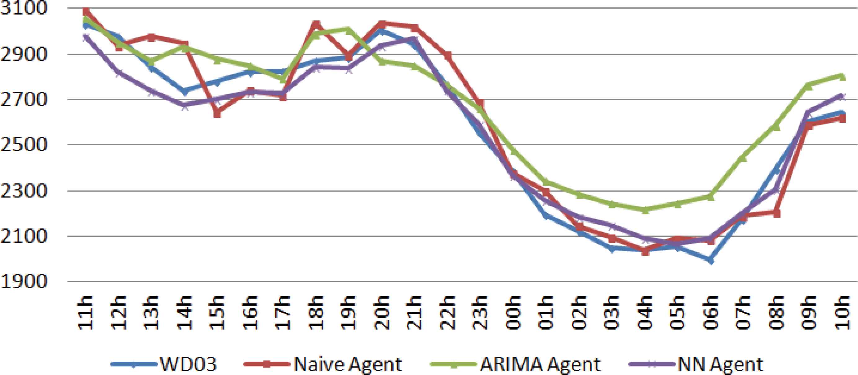
Testing period of the time series WD03: hourly water demand and forecasts (values in cubic meters).
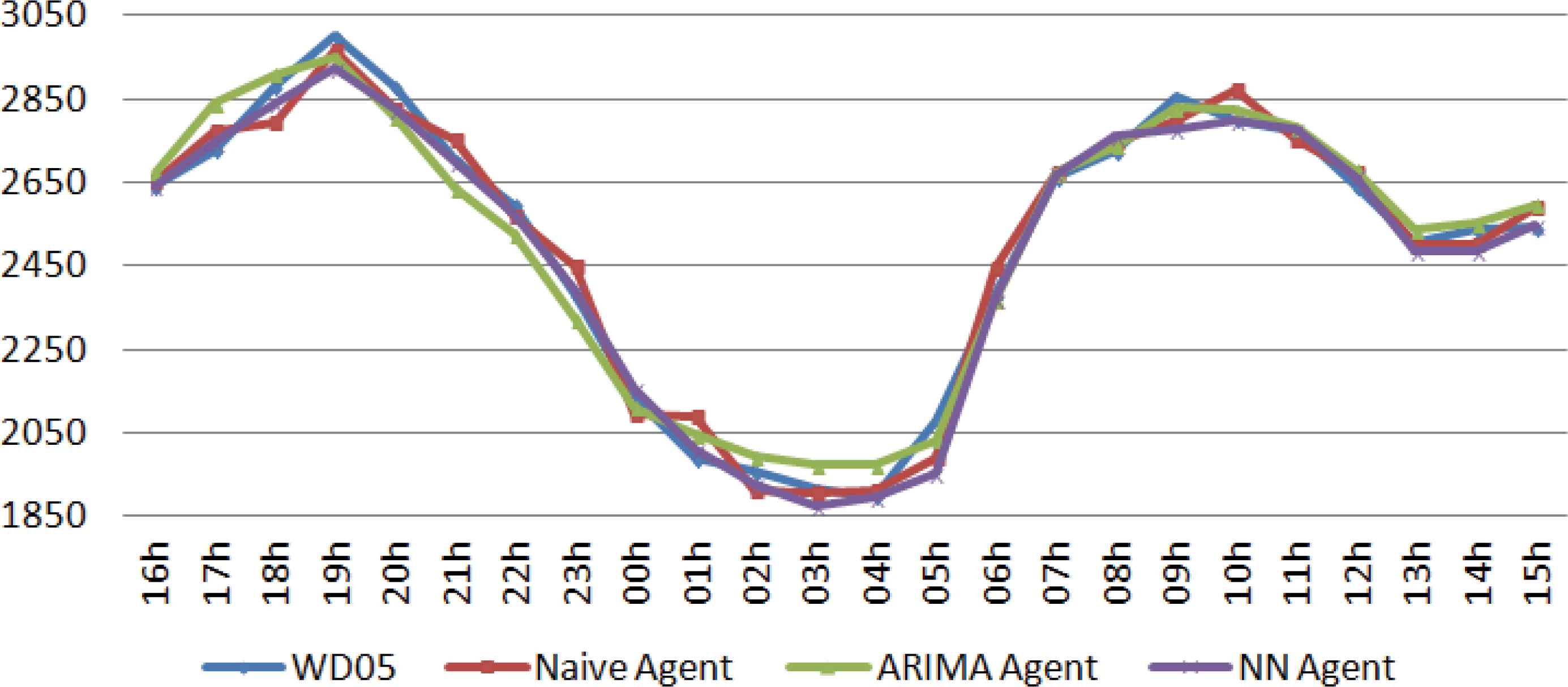
Testing period of the time series WD05: hourly water demand and forecasts (values in cubic meters).
4.2. Cost Overrun Reduction
The developed IDSS requires the introduction as an input of the unit cost overruns related to excessive storage and emergency water pumping. However, the really significant in terms of the solution provided by the system is the relationship between both according to Eq. (17). For this reason, the study of each series has been divided into three scenarios:
- (i)
Scenario 1: when both are equal (cewp=2 uc; cfw=2 uc),
- (ii)
Scenario 2: when the excessive storage overrun cost is three times the emergency water pumping overrun cost (cewp=1 uc; cfw=3 uc),
- (iii)
Scenario 3: when the relationship is the opposite (cewp=3 uc; cfw=1 uc).
Tables 3, 4 and 5 comprise the economic results of the tests in the three scenarios. That is to say, for each series, the costs of the solution provided by the MAS are shown. In order to compare the results, we have taken as a reference the solution provided by the base method. This tables contains the following data: the name of the series (Time Series); the WDM Cost Overrun in the testing period if the pumping system adjustment is made according to the base method (Cost Overrun Base Method); the forecasting agent that minimizes the overrun cost with the training data (Forecasting Agent); the WDM cost overrun in the testing period with the solution provided by the MAS (Cost Overrun MAS); and the percentage reduction achieved in comparison with the base method (Reduction Over Base Method).
| Time series | CO BM [*] | Forec. Agent | CO MAS | Reduct. over BM |
|---|---|---|---|---|
| WD01 | 1,094 | NN | 872 | 20.29% |
| WD02 | 2,730 | NN | 1,730 | 36.63% |
| WD03 | 10,022 | NN | 2,740 | 72.66% |
| WD04 | 3,338 | Naive | 1,872 | 43.92% |
| WD05 | 1,854 | NN | 1,416 | 23.62% |
| WD06 | 10,912 | Naive | 1,688 | 84.53% |
| WD07 | 2,906 | NN | 2,654 | 8.67% |
| WD08 | 2,276 | NN | 1,548 | 31.99% |
| WD09 | 2,844 | Naive | 1,718 | 39.59% |
| WD10 | 3,816 | NN | 910 | 76.15% |
| WD11 | 3,312 | NN | 3,230 | 2.48% |
| WD12 | 9,122 | MA | 2,786 | 69.46% |
CO: cost overrun
BM: base method.
Results of the MAS oriented to Minimizing Costs (In Units of Currency) for Scenario 1.
| Time series | CO BM [*] | Forec. Agent | CO MAS | Reduct. over BM |
|---|---|---|---|---|
| WD01 | 989 | NN | 720 | 27.20% |
| WD02 | 2,971 | NN | 1,967 | 33.79% |
| WD03 | 5,017 | NN | 2,394 | 52.28% |
| WD04 | 1,872 | Naive | 2,026 | −8.23% |
| WD05 | 2,577 | NN | 996 | 61.35% |
| WD06 | 7,136 | Naive | 1,574 | 77.94% |
| WD07 | 2,353 | ARIMA | 3,293 | −39.95% |
| WD08 | 3,036 | ES | 1,099 | 63.80% |
| WD09 | 3,358 | Naive | 1,659 | 50.60% |
| WD10 | 2,884 | NN | 767 | 73.40% |
| WD11 | 3,008 | NN | 3,665 | −21.84% |
| WD12 | 13,386 | MA | 2,675 | 80.02% |
CO: cost overrun
BM: base method.
Results of the MAS oriented to Minimizing Costs (In Units of Currency) for Scenario 2.
| Time series | CO BM [*] | Forec. Agent | CO MAS | Reduct. over BM |
|---|---|---|---|---|
| WD01 | 1,199 | ARIMA | 984 | 17.93% |
| WD02 | 2,489 | NN | 1,493 | 40.02% |
| WD03 | 15,027 | ES | 2,826 | 81.19% |
| WD04 | 2,640 | ARIMA | 1,267 | 52.01% |
| WD05 | 1,131 | ARIMA | 1,822 | −61.10% |
| WD06 | 14,688 | ES | 1,156 | 92.13% |
| WD07 | 3,459 | NN | 1,925 | 44.35% |
| WD08 | 1,516 | NN | 1,312 | 13.46% |
| WD09 | 2,330 | NN | 1,415 | 39.27% |
| WD10 | 4,748 | Naive | 819 | 82.75% |
| WD11 | 3,616 | NN | 2.795 | 22.70% |
| WD12 | 4,561 | NN | 2,460 | 46.07% |
CO: cost overrun
BM: base method.
Results of the MAS oriented to Minimizing Costs (In Units of Currency) for Scenario 3.
Results demonstrate the high efficiency of the system. The MAS for real-time WDM can achieve large reductions in cost overrun in comparison with the results obtained if the base method is used to adjust the pumping systems. In 32 of the 36 total tests, the system achieves a reduction in costs, and only in the remaining 4, the solution provided by the system would cause a higher cost. The average reduction is 42.50% for the first scenario, 37.53% for the second one, and 39.23% in the third scenario.
Moreover, these tables show that the choice of the forecasting method that results in the optimal alternative to adjust the pumping equipment varies according to the relationship between the cost overruns. For example, in WD03 series, ANN-based forecast generate the optimal setting in the first two cases, while in the latter the best forecast is provided by the ES Agent. Ten of the twelve series (all series except the WD02 and the WD11) clearly show this idea. Analyzing the previous tables in more detail (comparing it with Table 2), it can be observed that when the performance of a forecasting method is clearly superior to the others, the system tends to resort to it in order to minimize costs. However, when the difference is not very significant, choosing the best alternative to adjust the pumping depends on the ratio of costs. In these ten cases, an intermediate ratio could be found that differentiate the case when some forecasting method is optimal and the case when another is more appropriate.
These results confirm that limiting the study of WDM to the forecasting of this variable only implies finding a partial solution to the problem, which does not always lead to the best overall solution. It must be highlighted that WDM is a complex problem that should be understood as a whole and not as a collection of parts, and hence multi-agent techniques draw an appropriate framework to deal with it.
4.3. Pumping Systems Adjustment
As previously mentioned, the main output of the IDSS for real-time WDM is the optimal adjustment of the pumping systems. The system determines hourly the quantity of water to be pumped in order to minimize costs. As an example, Figure 9, based on the testing period of WD03, represents the solution proposed by the MAS for optimal adjustment of the pumping equipment in two opposite scenarios: when the excessive storage overrun cost is three times higher the emergency water pumping overrun cost (ANNs are used to forecast) and when the ratio is inverse (exponential smoothing is applied to forecast).
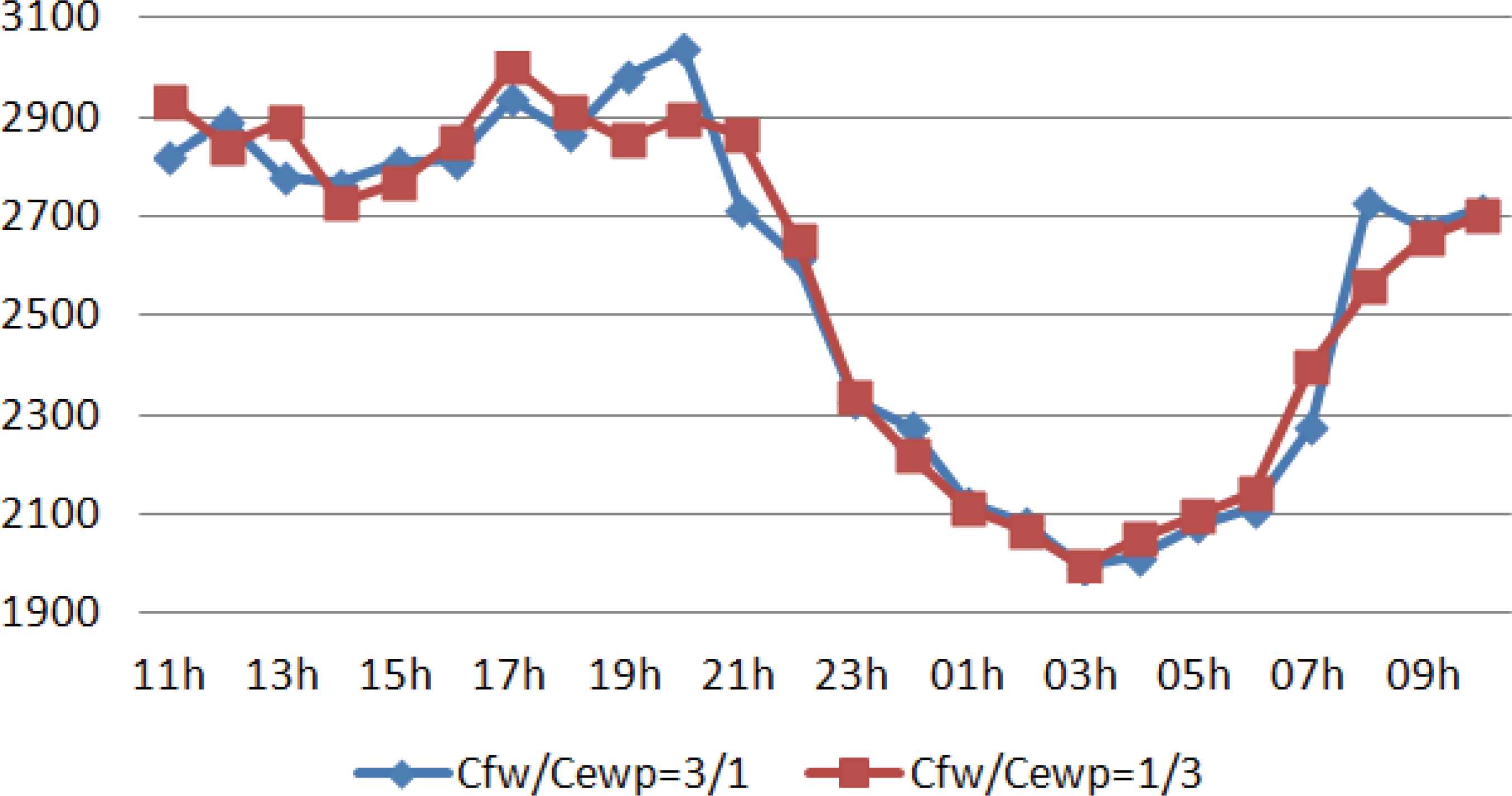
Testing period of the WD03 time series: optimal adjustment of the pumping system (values in cubic meters).
5. Conclusions and Future Work
This paper aims to show how the multi-agent methodology can be applied to WDM, a concept that has gained great importance in recent years given the requirements imposed by the new context marked by the scarcity of resources and the respect to the environment. In order to do this, an IDSS has been designed and implemented. It integrates sophisticated forecasting methods and management components under a structure that simulates a municipal water distribution system, and determines in real time the optimum adjustment of the pumping systems in order to minimize WDM costs.
Tests on time series with hourly water demand demonstrate the high efficiency of the developed system. They show that the introduction of AI techniques in the forecasting process, such as ANNs, can significantly decrease the error when compared with other traditional techniques, especially on holidays and days around them, because they have a greater capability of adapting to unexpected changes. This leads to a big reduction in WDM costs. However, the tests also show that the choice of the optimal alternative for adjusting the pumping systems depends on the input variables. Therefore, limiting the study to the search of the best forecasting method represents only a partial solution to the problem, which does not have to lead always to the best overall solution for the WDM system.
Again, it should be highlighted that this is a preliminary work or pilot system, where some simplified assumptions have been adopted (e.g. regarding the distribution system or the cost model). Translating this model into a real system would require reformulating these assumptions, as well as covering other common problems in real water distribution systems, such as leakages. In this regard, the main contribution of this work is that multi-agent methodology has proven to be not only a suitable tool to address this issue but also a necessary approach to study it, as WDM must be analyzed in its entirety from an holistic approach. In addition, this approach has enormous potential in increasing its functionality, as it allows managers to complete the study by adding new agents with the aim of increasing the scope of the system. It would also be possible to integrate this system into a MAS of greater magnitude.
Acknowledgements
This work has been carried out with financial support of the Government of the Principality of Asturias, through the Severo Ochoa program (ref. BP13011), and the Institute of Industrial Technology of Asturias (ref. SV-14-GIJON-1). Both are greatly appreciated, as well as the help provided by the Municipal Water Company of Gijón in providing data.
References
Cite this article
TY  - JOUR
AU  - Borja Ponte
AU  - David de la Fuente
AU  - José Parreño
AU  - Raúl Pino
PY  - 2016
DA  - 2016/01/18
TI  - Intelligent Decision Support System for Real-Time Water Demand Management
JO  - International Journal of Computational Intelligence Systems
SP  - 168
EP  - 183
VL  - 9
IS  - 1
SN  - 1875-6883
UR  - https://doi.org/10.1080/18756891.2016.1146533
DO  - 10.1080/18756891.2016.1146533
ID  - Ponte2016
ER  -