
A snapshot of image pre-processing for convolutional neural networks: case study of MNIST
- DOI
- 10.2991/ijcis.2017.10.1.38How to use a DOI?
- Keywords
- Classification; Deep learning; Convolutional Neural Networks (CNNs); preprocessing; handwritten digits; data augmentation
- Abstract
In the last five years, deep learning methods and particularly Convolutional Neural Networks (CNNs) have exhibited excellent accuracies in many pattern classification problems. Most of the state-of-the-art models apply data-augmentation techniques at the training stage. This paper provides a brief tutorial on data preprocessing and shows its benefits by using the competitive MNIST handwritten digits classification problem. We show and analyze the impact of different preprocessing techniques on the performance of three CNNs, LeNet, Network3 and DropConnect, together with their ensembles. The analyzed transformations are, centering, elastic deformation, translation, rotation and different combinations of them. Our analysis demonstrates that data-preprocessing techniques, such as the combination of elastic deformation and rotation, together with ensembles have a high potential to further improve the state-of-the-art accuracy in MNIST classification.
- Copyright
- © 2017, the Authors. Published by Atlantis Press.
- Open Access
- This is an open access article under the CC BY-NC license (http://creativecommons.org/licences/by-nc/4.0/).
1. Introduction
The task of classification in automatic learning consists of extracting knowledge from a set of labeled examples in order to acquire the ability to predict the correct label of any given instance 1. A fundamental aspect of a good classifier is its ability to generalize on new data, i.e., correctly classify new instances that do not belong to the training set.
In the last five years, deep learning in general and Convolutional Neural Networks (CNNs) in particular have demonstrated a superior accuracy to all the classical methods in pattern recognition, classification and detection specially in the field of computer vision. In fact, since 2012, the prestigious Large Scale Visual Recognition Challenge (ILSVRC) has been won only by CNNs 2. Two of the main reasons behind this success is i) the emergence of new large labeled databases such as, ImageNet (http://image-net.org/), and also ii) the advances in GPU (Graphics Processor Unit) technology, which have made this device ideal for accelerating the convolution operations involved in CNNs. CNNs are showing a high potential for learning more and more complex patterns 2. They have been used with success in diverse problems, e.g., image classification 2,3, handwritten digit recognition 4 and speech recognition 5,6, and they are being explored in more fields and applications.
Data preprocessing 7 is an essential part of any automatic learning process. In some cases, it focuses on correcting the deficiencies that may damage the learning process, such as omissions, noise and outliers 8. In other cases, it focuses on adapting the data to simplify and optimize the training of the learning model.
In contrast to the classical classification models, the high abstraction capacity of CNNs allows them to work on the original high dimensional space, which reduces the need for manually preparing the input. However, a suitable preprocessing is still important to improve the quality of the results 9.
One of the most used preprocessing techniques with CNNs is data augmentation, which increases the volume of the training dataset by applying several transformations to the original input 2,4,10. Data augmentation replicates the instances of the training set by introducing various types of transformations, e.g., translation, rotation, several types of symmetries, etc. Such techniques decrease the sensitivity of the training to noise and overfitting.
MNIST is a handwritten digit database 11 that contains 60,000 training instances and 10,000 test instances. Each instance is a 28 × 28 single channel grayscale image. MNIST has been written by different persons to avoid correlations. The 70,000 images are distributed into 10 classes, one class per digit, from 0 to 9. Each class has approximately the same number of instances. The updated classification results for MNIST can be found in 11,12.
This paper analyzes different preprocessing and augmentation techniques for CNNs using as case study the problem of handwritten digit classification. We focus on analyzing combinations of these transformations: centering, translation, rotation and elastic deformation. The objective is to evaluate to which extent these transformations affect the results of CNNs on the widely used MNIST dataset 11. We consider the following well known networks, LeNet 4, Network3 13 and DropConnect 14. The latter network represents the current state-of-the art for MNIST classification.
This document is organized as follows: First, section 2 presents the general features of deep learning for classification including a brief description of CNNs, ensembles and deep learning software. Section 3 describes the data preprocessing techniques studied in this work together with the state-of-theart models in MNIST classification. Section 4 describes the CNNs we used for the problem of handwritten digits recognition. Section 5 provides the experimental setup. Section 6 shows the experiments we carried out for this work and the analysis of the results. Finally, section 7 outlines the conclusions.
2. Deep learning for classification
This section provides an introduction to deep learning and CNNs and describes the CNNs used for handwritten digits classification.
2.1. Brief introduction to deep learning and CNNs
There exist several types of neural networks. In this work we focus on feed-forward Convolutional Neural Networks for supervised classification, as they provide very good accuracies for MNIST. A CNN is formed by a set of layers of neurons, each neuron is connected to the neurons of the previous layer by a vector of weights, so that the value of a neuron is computed as a weighted sum of the neurons from the previous layer. Neurons can apply an activation function to introduce non-linearity.
The classification mechanism works as follows: it uses the instance that we intend to classify to set the values of the first layer of the network (input layer). Then, these values are propagated along the multiple layers of the CNN until the final layer (output layer), which outputs the predicted class. In general, each layer extracts a certain level of abstraction.The first layers capture low-level features, e.g., edges, and the deeper layers capture high-level features, e.g., shapes specific to one class. Therefore, the larger the number of layers, the higher is the learning capacity of more complex and generic patterns 15. There exist three different types of layers in a CNN 4,15:
- •
Fully connected layers: each neuron is connected by weights to all neurons of the previous layer.
- •
Convolutional layers: each neuron is connected to a smaller area of neurons, called patch, in the previous layer. In this type of layers, the weights are shared among all neurons of the same layer, which reduces the search space of the learning process.
- •
Pooling layers: usually located after a convolutional layer. Similarly to convolution layers, each neuron is connected to an area of the previous layer, and computes the maximum or average of those values.
In practice, CNNs include combinations of these three types of layers. For illustration see the CNN example shown in Figure 1. These networks are adapted to extract knowledge from images and structures that include some sort of spatial pattern, as demonstrated by the results in diverse competitions 2,17.
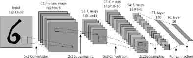
Types of layers 16 that constitute LeNet CNN architecture.
When a network is used to classify a problem of m classes, c1, …, cm, the output layer outputs one neuron per class, i.e., a vector a = (a1, …, am). We have used the SoftMax function to convert these values into probabilities (equation 1), where SoftMax(ai) is the probability that the input belongs to class ci. Therefore, the CNN-model will intend to output m − 1 neurons with values close to zero, except for the correct class, which should be closed to 1.
The training of a network involves optimizing the weights of each neuron until the network acquires the ability of predicting the correct label for each input. The dimensions of the search space are as many as the total number of weights. The reference algorithm for training neural networks is the Gradient Descent (GD) algorithm with back propagation 18. GD computes the output of the network for all the training examples, then, computes the output error and its derivatives with respect to the weights to finally update the weights in the desired direction. GD iterates over the whole training set multiple times until convergence. The magnitude of the change of the weights is called learning rate.
Training CNNs is computationally expensive due to the large search space and complexity of the training algorithm. Alternatively, Stochastic Gradient Descent (SGD) algorithm reduces these limitation by using only a subset, called batch, of the training set in each iteration. Although the error function is not well minimized as in the case of GD. An iteration over the entire training set, called epoch, requires multiple iterations over the small batches. This algorithm along with the recent advances in GPUs and the availability of larger datasets have allowed training deep CNNs successfully and with very good results.
The SGD is often combined with complementary operations to improve the convergence and generalization of the network:
- •
Momentum 19: the direction in which the weights line is updated is a linear combination of the previous search direction and the one obtained with the current batch. This avoids part of the bias introduced by each batch to keep a steadier direction throughout the search process.
- •
Adam (Adaptive Moment Estimation) 20: a stochastic optimization technique that computes individual adaptive learning rates for different parameters from estimates of first and second moments of the gradients.
- •
Dropout 21: for each training set, it randomly omits a selected subset of feature detectors by setting the layer’s output units to 0. Dropconnect 14 is a generalization of dropout, it randomly sets a selected subset of weights (i.e., connections) instead of output vectors to 0. Both, dropout and dropconnect are used for regularizing large fully connected layers with the objective to reduce overfitting.
- •
ReLU (Rectified Linear Units) 22: these units are linear when their input is positive and zero otherwise. ReLU makes training deep networks faster than using standard sigmoid units. It also improves the generalization of deep neural networks.
- •
Normalization: the sum of the weights (or their squares) is added to the error function to improve the robustness of the learning process.
2.2. CNNs and ensembles for handwritten digits classification
Several previous works have shown that selecting a complete set, i.e., ensemble, of the best performing networks and running them all with an appropriate collective decision strategy increases the performance 23,24. This is due to the fact that the computation of the weights is an optimization problem with many local minima.
In this work we have analyzed the impact of the preprocessing on both, single CNNs based-models and ensembles of CNNs based-models.
As mentioned before, we have selected three models with similar architectures, LeNet 4, Network3 13 and DropConnect 14. The three models have shown very good accuracies on handwritten digit classification. LeNet, consists of two convolutional layers (each one followed by max pooling) and two fully connected layers (see Table 1). The Cross Entropy is used as loss function and the output layer outputs 10 neurons with SoftMax activation function.
| Layer | Filter size for | Stride | Activation | |
|---|---|---|---|---|
| 28×28-input | 20×20-input | |||
| conv1 | 5 × 5 × 20 | 7 × 7 × 20 | 1/3 | – |
| maxpool1 | 2 ×2 | 2 ×2 | 2 | – |
| conv2 | 5 ×5×50 | 5 ×5×50 | 1 | – |
| maxpool2 | 2 ×2 | 2 ×2 | 2 | – |
| fc1 | 500 | 500 | – | ReLU |
| fc2 | 10 | 10 | – | SoftMax |
Topology of LeNet. Columns 2 and 3 show the configuration for processing original and cropped input images respectively.
Similarly, Network3, consists of two convolutional layers (each one followed by max pooling) and three fully connected layers (see Table 2) with rectified linear units activation instead of sigmoid one. The Cross Entropy is used as loss function and the output layer outputs 10 neurons with SoftMax activation function. Both architectures have been trained using SGD algorithm.
| Layer | Filter size for | Stride | Activation | |
|---|---|---|---|---|
| 28×28-input | 20×20-input | |||
| conv1 | 5 × 5 × 20 | 3 × 3 × 20 | 1 | relu |
| maxpool1 | 2 ×2 | 2 × 2 | 2 | – |
| conv2 | 5 × 5 × 40 | 2 ×2×40 | 1 | relu |
| maxpool2 | 2 × 2 | 2 ×2 | 2 | – |
| fc1 | 640 | 640 | – | relu & dropout rate=0.5 |
| fc2 | 1000 | 1000 | – | relu & dropout rat =0.5 |
| fc3 | 10 | 10 | – | SoftMax |
Topology of Network3 13. Columns 2 and 3 show the configuration for processing original and cropped input images respectively.
DropConnect 14, is similar to the previous ones. The main difference is that it uses dropconnect optimization in the first fully connected layer (see Table 3).
| Layer | Filter size for | Stride | Activation | |
|---|---|---|---|---|
| 28×28-input | 20×20-input | |||
| conv1 | 5 × 5 × 32 | 7 × 7 × 32 | 1/3 | – |
| maxpool1 | 2 ×2 | 2 × 2 | 2 | – |
| conv2 | 5 ×5 ×64 | 5 × 5 × 64 | 1 | – |
| maxpool2 | 2 × 2 | 2 ×2 | 2 | – |
| fc1 | 150 | 150 | – | relu & drop-connect rate: 0.5 |
| fc2 | 10 | 10 | – | softMax |
Topology of DropConnect 14. Columns 2 and 3 show the configuration for processing original and cropped input images respectively.
2.3. Deep learning software
The high interest in deep learning, shown in industry and Academia, has involved the development of a large number of software to ease the creation, reutilization and portability of deep learning codes. As the field of deep learning is still evolving, there is no standard library for building deep learning based models. All the existent software are still under development, i.e., they do not support all the optimizations, for example, dropconnet is not supported yet by most libraries. The existent software can be classified in different ways, e.g., in terms of, target applications, used programming languages 25 and target computing systems.
For the problem analyzed in this work, we have considered Caffe 26, Theano 27 and cuda-convnet 28.
Caffe (Convolution Architecture For Feature Extraction) is a framework, with a user friendly interface, that provides several examples and models, e.g., Alexnet, googlenet and RNN, for training deep learning models on well known datasets. One of the interesting aspects in Caffe is that it allows fine-tuning, which consists in taking an already learned model, adapts the architecture and resume training from the already learned model weights. It is coded using C++ and CUDA and provides Command line, Python and MATLAB interfaces. Caffe can be accelerated using one or multiple GPUs.
Theano is a Python library for handling mathematical expressions with multi-dimensional numerical arrays. It does not provide pre-built models or examples as in Caffe. Although we have used pure Theano in this work, in general, it is not used directly for building deep learning models. Instead Theano is used as backend for more specialized and user friendly frameworks such as, Lasagne and Keras. The training and testing on Theano can also be accelerated using GPUs.
Cuda-convnet 28 is a deep learning framework implemented with C++ and CUDA. It allows implementing convolutional feed-forward neural networks and modeling arbitrary layer connectivity and network depth. Currently, Cuda-convnet is the only deep learning Software that supports dropconnect operation. The training is done using the back-propagation algorithm. Cuda-convnet can be accelerated using single and multiple GPUs. It is worth to mention that Cuda-convnet is not maintained since 2014. None of the considered deep learning software, i.e., Theano, Caffe and DropConnet, provide support for ensembles.
The deep learning popularity results in numerous open-source software tools. For readers with interest in deep learning software tools, in 29 we can find an interesting experimental analysis on CPU and GPU platforms for some well known GPU-accelerated tools, including: Caffe (developed by the Berkeley Vision and Learning Center), CNTK (developed by Microsoft Research), Tensorflow (developed by Google) and Torch.
3. Preprocessing handwritten digits
This section first explains the preprocessing techniques used in this work and gives a description of the top-5 most accurate networks for classifying MNIST database.
3.1. Preprocessing and augmentation
We have applied the different preprocessing methods to increase the performance of CNN models. The main purpose of these methods is making learning algorithms invariant to some transformations of the images. Translations, rotations and elastic deformations methods have already been studied for different purposes in the field of automatic learning 4,15,10. These methods apply a predefined transformation to each image, obtaining new instances for the training set. We also propose a centering method, which does not need to increase the dataset size in order to make learning algorithms invariant to translations. We discuss each of these methods separately.
- •
Translations: The image is translated a number of pixels toward a given direction.
- •
Centering: This method is applied to the training and the test sets. First, the white rows and columns are eliminated from the borders of each image. This process may produce images of different sizes. Afterwards, the maximum number of rows (rmax) and columns (rmax) of the cropped images are calculated. Finally, all the images are re-sized by scaling them to the same size rmax × cmax. This preprocessing approach removes parts of the image that do not provide useful information, making the learning process faster. Furthermore, the resizing step normalizes the digits scale and, hence, equal digits are more similar to each other. When centering is combined with other transformations, the centering is applied at the end of the preprocessing so that the final images will be centered. Note that translations and centering methods shouldn’t be applied together.
- •
Rotations: The image is rotated to a given angle θ. The center of the rotation is the center of the image, denoted (a, b). The rotation is given by
However, since we are dealing with maps of pixels rather then vectorial images, it is necessary to apply interpolations when computing the rotation. Concretely, for each pixel (i, j) in the resulting image we compute the pixel’s value as the bilinear interpolation of the original pixels surrounding Φ−θ (i, j). Note that interpolations increase the variability of the resulting images. - •
Elastic deformation: Image pixels are slightly moved in random directions, keeping the image’s topology. This transformation imitates the possible variability which takes place when one writes the same digit twice. An elastic deformation is obtained as follows: For each pixel (i, j) in the resulting image we compute its location in the original image, denoted (i′, j′). The original location is determined by the displacement matrices ∆x and ∆y, (i′, j′) = (i + ∆y(i, j), j + ∆x(i, j)). Afterwards, the pixel value is obtained on applying a bilinear interpolation. The remaining problem is determining the displacement matrices. Algorithm 1 gives a method to compute them. Initially, the displacement matrices are initialized with random values between −α and α using an uniform distribution, where α is the deformation strength in pixels. If we use these displacement matrices, then the resulting image will be extremely different from the original one. Thus, a convolution with a gaussian kernel is applied, that is, each component is recomputed as a weighted average of all the matrix components, where the weights are given by a two-dimensional Gaussian function
The standard deviation σ determines the weights. If σ is small, then the rest of the components have small weights and, hence, the transformation is mostly random. On the other hand, if σ is large, then the weights are similar to each other and, thus, the transformation is likely a translation. Consequently, values around σ = 6 are used in the specialized literature 10.
| Require: The matrix dimension n, the displacement strength α and the standard deviation σ. |
| 1: ∆ ← n × n matrix with random components between −α and α. |
| 2: for i = 1,2,... n do |
| 3: for j = 1, 2, n do |
| 4: |
| 5: end for |
| 6: end for |
| 7: return ∆ |
Random Displacement Matrix
Figure 2 shows three examples from MNIST, together with their respective centering transformations (2nd column), elastic deformation (3rd column), translation (4th column) and, rotation (5th column). Figure 3 shows the average value of 10 original images from MNIST and the resulting images before and after applying the centering algorithm.
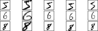
Three original MNIST images (1st column) and the obtained images after centering (2nd column), elastic deformation (3rd column), translation (4th column) and rotation (5th column).
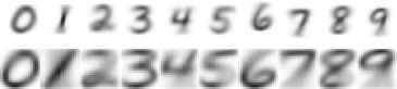
Average value of 10 images from MNIST, one image per class, before and after applying the centering process.
The transformations described in this section, i.e., rotation, translation, elastic deformation and centering, can be combined together to further increase the volume and variability of the dataset used for training the network. Table 4 shows the set of preprocessing combinations analyzed in this work, along with the number of instances that form each training set. Note that the datasets of the combinations from 3 to 12 include also the original images without transformations.
| Dataset | Combination | # of training instances |
|---|---|---|
| 1 | Original | 60,000 |
| 2 | Centering | 60,000 |
| 3 | Elastic | 300,000 |
| 4 | Translation | 300,000 |
| 5 | Rotation | 300,000 |
| 6 | Elastic-centering | 300,000 |
| 7 | Rotation-centering | 300,000 |
| 8 | Translation-elastic | 1,500,000 |
| 9 | Translation-rotation | 1,500,000 |
| 10 | Rotation-elastic | 1,500,000 |
| 11 | Rotation-elastic-centering | 1,500,000 |
| 12 | Elastic-elastic | 1,500,000 |
The combinations of transformations analyzed in this study. All the combinations, from dataset 3 to 12, include the original dataset.
3.2. MNIST classification: Using data augmentation to get the state-of-the-art results
Although the focus of this paper is to analyze the impact of the pre-processing on CNNs based models, this section provides an overview of the most accurate models for MNIST classification. Notice that the three most accurate models for MNIST classification use data-augmentation.
The ranking of the 50 most accurate models for classifying handwritten digits can be found in 12. Each model attempts to minimize the test error by introducing new optimizations. As summarized in Table 5, the top-5 models are:
- •
The fifth most accurate model 30 obtains a test error, 0.29%, without data augmentation by replacing the typical, max or average, pooling layer with a gated max-average pooling.
- •
Maxout network In Network (MIN) model 31 reaches a test accuracy, 0.24%, without data augmentation by applying a batch normalization to the maxout units of the model.
- •
APAC-based Neural Networks 32 obtains a test error, 0.23%, by 1) introducing a new decision rule for augmented dataset, which basically consists in calculating the mean of logarithm of the softmax output and, 2) preprocessing the training set using elastic distortions.
- •
The multi-column deep neural networks model 33 provides a test accuracy similar to the previous one, 0.23%, by calculating the final prediction of each test as the average of the predictions of the deep learning model trained on input preprocessed in different ways, translated, scaled, rotated and elastically distorted.
- •
DropConnect network 14 obtains the state-of-theart test error, 0.21%, by 1) applying dropout optimization to the weights instead of the activation units, 2) preprocessing the training dataset (crop, rotate and scale the images then subtract the image mean), 3) training the network using the 700-200-100 epoch schedule as follows: Using three training stages, 700 epochs, 200 epochs and 100 epochs, and different multipliers for each stage. Multiplying the initial learning rate by 1 in the first stage. Multiplying the rate by 0.5 and train the net 200 epochs and again multiply the rate by 0.1 and retrain during 200 epochs. Multiplying the rate by 0.05, 0.01, 0.005 and 0.001 and train 100 epochs successively 4) using an ensemble of 5 networks trained on different sequences of random permutations of the training set using the most voted strategy.
| Model | Test error | published in |
|---|---|---|
|
|
||
| DropConnet 14 | 0.21% | ICML 2013 |
| Multi-column deep neural networks 33 | 0.23% | CVPR 2012 |
| APAC Neural Networks 32 | 0.23% | arXiv 2015 |
| MIN(Maxout network In Network) 31 | 0.24% | arXiv 2015 |
| CNNs with generalized pooling functions 30 | 0.29% | AISTATS 2016 |
Test errors (in %) reported by the five most accurate models for MNIST classification.
4. Experimental analysis
This section presents and analyzes the impact of the preprocessing techniques, described in section 3.1, on the performance, in terms of accuracy, which is the most used metric in MNIST problem, and execution time, of LeNet, Network3 and DropConnect. We will also analyze the impact of the preprocessing on several ensembles combined with different decision strategies and on Net configurations.
4.1. Experimental setup
The three considered convolutional networks, LeNet, Network3 and DropConnect are implemented respectively in Caffe 26, Theano 27 and Cuda-convnet2 28. Table 6 shows the parameters used for the data preprocessing and for the training.
| Algorithm | Parameter | Value |
|---|---|---|
|
|
||
| LeNet (SGD) | Number of iterations | 10,000 / 50,000 |
| Batch size | 64 / 256 | |
| Learning rate | lr0(1 + γ * iter)−b | |
| Initial learning rate (lr0) | 0.01 | |
| γ | 0.0001 | |
| b | 0.75 | |
| Momentum | 0.9 | |
| Regularization Coefficient L2 | 0.0005 | |
|
|
||
| Network3 (SGD) | Number of epochs | 10 / 20 |
| minibatch size | 10 | |
| Learning rate | 0.03 | |
| γ | 0.0001 | |
|
|
||
| DropConnect (SGD) | Number of epochs | 100 / 200 |
| minibatch size | 128 | |
| Learning rate | 0.01 | |
| Momentum | 0.9 | |
|
|
||
| Elastic transformation | Typical deviation | 6 |
| Number of transformations | 4 | |
| Strength | 4 | |
|
|
||
| Translation | Magnitude | ±3 pixels |
| Direction | Vertical y horizontal | |
|
|
||
| Rotation | Angles | ±8 y ±16 degrees |
|
|
||
| Centering | Final size | 20 ×20 pixels |
Parameters of the used learning models and preprocessing algorithms
4.2. Preprocessing analysis
This section presents and analyzes the impact of all the considered preprocessing technique on the accuracy of LeNet, Network3 and DropConnect. The average and best test accuracies shown in this section are measured as follows. For each training set, the average accuracy is calculated as the average of the final accuracies obtained over 5 executions of the considered learning model. The best accuracy is the highest final accuracy over the 5 executions.
4.2.1. LeNet
Table 7 shows the results of LeNet on the twelve considered preprocessed training sets using 10,000 and 50,000 iterations. The results are expressed in terms of, average and best test accuracies. The highest accuracy in each column is highlighted in bold and the best top five accuracies are labeled as 1, 2, 3, 4 and 5. Recall that in Caffe, Epoch is calculated as
| LeNet (10,000 iter.) | LeNet (50,000 iter.) | |||||||
|---|---|---|---|---|---|---|---|---|
| Dataset | Average | Best | Epochs | Time(s) | Average | Best | Epochs | Time(s) |
| Original | 99.08% | 99.18% | 10.67 | 267.91 | 99.05% | 99.21% | 213.33 | 1070.29 |
| Centered | 98.85% | 99.06% | 10.67 | 203.52 | 98.95 % | 98.09% | 213.33 | 926.38 |
| Elastic | 99.09% | 99.19% | 2.13 | 232.75 | 99.36% | 99.44% | 42.67 | 1065.38 |
| Translation | 99.09% | 99.32% | 2.13 | 268.75 | 99.30% | 99.41% | 42.67 | 1065.38 |
| Rotation | 99.05% | 99.10% | 2.13 | 268.03 | 99.25% | 99.37% | 42.67 | 1065.38 |
| Elastic-centered | 599.17% | 99.26% | 2.13 | 267.20 | 99.27% | 99.36% | 42.67 | 925.51 |
| Rotation-centered | 98.90% | 99.07% | 2.13 | 232.73 | 99.19% | 99.33% | 42.67 | 950.38 |
| Translation-elastic | 499.18% | 99.32% | 0.43 | 267.43 | 599.39% | 99.54% | 8.53 | 1050.38 |
| Translation-rotation | 99.16% | 99.40% | 0.43 | 267.41 | 399.40% | 97.55% | 8.53 | 1045.38 |
| Rotation-elastic | 199.31% | 99.39% | 0.43 | 268.14 | 199.47% | 99.57% | 8.53 | 1046.25 |
| Rotation-elastic-centered | 399.19% | 99.24% | 0.43 | 232.30 | 299.43% | 99.52% | 8.53 | 925.68 |
| Elastic-elastic | 299.27% | 99.45% | 0.43 | 268.10 | 499.40% | 99.50% | 8.53 | 1047.64 |
Average and best test accuracies obtained by LeNet on each one of the preprocessed datasets using 10,000 and 50,000 iterations. Time (columns 5 and 9) is the time taken to execute the training-testing process on each dataset. The top five accurate models are labeled as 1, 2, 3, 4 and 5.
In general, except for the case of centered set, training LeNet on a pre-processed training set always leads to better accuracies than training it on the non-preprocessed one, i.e., the original set. In addition, the convergence of LeNet is always faster on the pre-processed sets. The five most accurate result using 10,000 iterations are obtained in order by, the rotation-elastic, elastic-elastic, rotation-elastic-centered, translation-elastic and elastic-centered sets. The five most accurate result using 50,000 iterations are obtained in order by, the rotation-elastic, rotation-elastic-centered, translation-rotation, elastic-elastic and translation-elastic sets. The best accuracy, 99.47%, is obtained by the rotation-elastic pre-processing using 50,000 iterations. A remarkable result is that the best accuracy for 10,000 iterations is obtained with only 0.43 epochs, which means that only 43% of the dataset instances has been used for the training, where each instance has been used only once.
4.2.2. Network3
Table 8 shows the average and best test accuracies of Network3 on the twelve considered preprocessed datasets using 10 and 50 epochs. The five most accurate results for 10 epochs are obtained in order by, the elastic-elastic, rotation-elastic, translation-rotation, translation-elastic and translation sets. The five most accurate results for 20 epochs are obtained in order by, elastic-elastic, rotation-elastic, elastic, translation and translation-elastic sets. The best accuracy, 99 67%, is obtained by the elastic-elastic pre-processing method using 20 epochs. Similarly to LeNet, except for the case of centered set, training Network3 on a pre-processed training set always leads to better accuracies than training it on the original training set. In addition, the convergence of Network3 is always faster on the pre-processed sets.
| Network3(10 epochs) | Network3(20 epochs) | |||||
|---|---|---|---|---|---|---|
| Dataset | Average | Best | Time(s) | Average | Best | Time(s) |
| Original | 99.01% | 99.07% | 124.45 | 99.25% | 99.25% | 205,21 |
| Centered | 98.73% | 98.80% | 118.32 | 98.97% | 99.01% | 196.92 |
| Elastic | 99.49% | 99.54% | 656,85 | 399.61% | 99.67% | 1200,33 |
| Translation | 599.49% | 99.55% | 631.53 | 499.59% | 99.63% | 1228,71 |
| Rotation | 99.44% | 99.50% | 636.25 | 99.44% | 99.50% | 1256,95 |
| Elastic-centered | 99.32% | 99.39% | 566.44 | 99.57% | 99.60% | 1109,43 |
| Rotation-centered | 98.88% | 98.94% | 569.04 | 99.31% | 99.32% | 1167,32 |
| Translation-elastic | 499.54% | 99.57% | 3647.78 | 599.58% | 99.63% | 7111,65 |
| Translation-rotation | 399.57% | 99.61% | 3650.66 | 99.58% | 99.60% | 7149,25 |
| Rotation-elastic | 299.62% | 99.67% | 3642,85 | 299.67% | 99.69% | 6996,23 |
| Rotation-elastic-centered | 99.43% | 99.51% | 3054,43 | 99.51% | 99.52% | 6908,70 |
| Elastic-elastic | 199.65% | 99.66% | 3607.32 | 199.67 % | 99.70% | 7189,16 |
Average and best test accuracies obtained by Network3 on the twelve datasets using 10 and 20 epochs. Time (columns 5 and 9) is the time taken to train Network3 on each dataset. The top five accurate models are labeled as 1, 2, 3, 4 and 5.
4.2.3. DropConnect
As our focus is not improving the state-of-the-art error, we have analyzed the accuracy of DropConnect network using shorter training periods, 10 and 20 epochs. Recall that to reach the current state-of-the-art error, 0.21%, reported in 14, the authors employed the 700-200-100 cascade schedule.
Table 9 shows the results of DropConnect on the considered preprocessed datasets using 10 and 20 epochs. The five most accurate results for 10 epochs are obtained in order by the elastic-elastic, translation-rotation, rotation-elastic, translation-elastic-centered and translation sets. The five most accurate results for 20 epochs are obtained in order by, the translation-rotation, elastic-elastic, translation-elastic, rotation-elastic and translation sets. The best accuracy, 99.69%, is obtained by the translation-rotation training set using 20 epochs. As it can be seen from Tables 7, 8 and 9 the best performance of each network is obtained by a different pre-processing techniques. DropConnet provides the highest accuracy over the three evaluated networks.
| DropConnet(100 epochs) | DropConnet(200 epochs) | |||||
|---|---|---|---|---|---|---|
| Dataset | Average | Best | Time(s) | Average | Best | Time(s) |
| Original | 98,32% | 98,83% | 7803.43 | 98.98% | 98,99% | 18748.53 |
| Centered | 95.35% | 94,46% | 6659.31 | 95.13% | 98,85% | 18635.54 |
| Elastic | 99.33 % | 99,35% | 7512.25 | 99.36% | 99,36% | 18606.15 |
| Translation | 599.43% | 99,46% | 7736.41 | 599.47% | 99,47% | 18710.45 |
| Rotation | 99.18% | 99,29% | 7151.73 | 99.37% | 99,47% | 18729.29 |
| Elastic-centered | 96.58% | 96,69% | 6969.89 | 97.08% | 97,09% | 18661.80 |
| Rotation-centered | 98.30% | 98,41% | 6974.23 | 98.55% | 98,63% | 18668.05 |
| Translation-elastic | 99.40% | 99,57% | 7162.37 | 399.58% | 99,58% | 18745.93 |
| Translation-rotation | 299.57% | 99,59% | 7410.32 | 199.69% | 99,69% | 18772.40 |
| Rotation-elastic | 399.54% | 99,60% | 7397.40 | 499.56% | 99,56% | 18724.38 |
| Rotation-elastic-centered | 499.47% | 99,49% | 7803.73 | 99,44% | 99,46% | 18220.50 |
| Elastic-elastic | 199,58% | 99,59% | 7911.30 | 299,59% | 99,61% | 18712.22 |
Average and best test accuracies obtained by DropConnect on the twelve datasets using 100 and 200 epochs. Time (columns 5 and 9) is the time taken to execute the training-testing process on each dataset. The top five accurate models are labeled as 1, 2, 3, 4 and 5.
4.2.4. Different configurations of LeNet fully Connected layer
This subsection illustrates the impact of dropout operation on the performance of LeNet. Table 10 shows the accuracies obtained by different configurations of the 1st Fully Connected Layer of LeNet, 500 neurons (the configuration used for the experiments shown in Table 7), 1000 neurons and, 1000 neurons combined with dropout. In general, the configuration with 1000 neurons combined with dropout provides the best accuracies over the first two configurations for all the preprocessing datasets.
| Dataset | 500 neurons | 1000 neurons | 1000 neurons+ dropout |
|---|---|---|---|
|
|
|||
| Original | 99,05% | 99,05% | 99,24% |
| Centered | 98,95% | 98,98% | 99,16% |
| Elastic | 99,36% | 99,35% | 99,46% |
| Translation | 99,30% | 99,29% | 99,45% |
| Rotation | 99,25% | 99,26% | 99,37% |
| Elastic-centered | 99,27% | 99,33% | 99,41% |
| Rotation-centered | 99,19% | 99,15% | 99,37% |
| Translation-elastic | 99,39 % | 99,39% | 99,49% |
| Translation-rotation | 99,40% | 99,40% | 99,49% |
| Rotation-elastic | 99,47% | 99,50% | 99,55% |
| Rotation-elastic-centered | 99,43% | 99,48% | 99,48% |
| Elastic-elastic | 99,40% | 99,50% | 99,53% |
Test accuracies of LeNet with 500, 1000 and 1000 with dropout.
4.2.5. Ensembles
This section analyzes the impact of the preprocessing on different ensembles, different configurations and different training durations. We will first analyze the effect of different configurations and decision criteria on Lenet-based ensembles then we will show the performance of ensembles of Lenet, Network3 and DropConnect using the most voted decision strategy, which is the strategy used for MNIST classification in 14.
Table 11 shows the accuracies obtained by two ensembles made up of the five and three best models, ensemble-5 and ensemble-3, based on LeNet, with different 1st fully connected layer configurations, and using different decision strategies, the most voted strategy (MV), the maximum of probability summation (MPS) and the maximum probability (MP). In general, ensemble-5 and -3 provide better accuracies over all individual models from Table 7. The best accuracy, 99,68%, is obtained by the configuration 1000 neurons with dropout using the maximum of probability summation strategy.
| LeNet | |||||||||
|---|---|---|---|---|---|---|---|---|---|
|
|
|||||||||
| 500 neurons | 1000 neurons | 1000 neurons with dropout | |||||||
| MV | PSM | MP | MV | PSM | MP | MV | PSM | MP | |
| Ensemble-5 | 99,57% | 99,56% | 99,59% | 99,60% | 99,62% | 99,63% | 99,61% | 99,64% | 99,63% |
| Ensemble-3 | 99,54% | 99,58% | 99,62% | 99,61% | 99,66% | 99,64% | 99,65% | 99,68% | 99,64% |
Test accuracies obtained by ensemble-5 and ensemble-3, using three configurations of the 1st fully connected layer of Lenet, based on three decision strategies, the most voted strategy (MV), the maximum of probability summation (MPS) and the maximum probability (MP).
Network3 and DropConnect codes do not provide the weights associated to each class. Therefore, for the next results we have employed only the most voted decision strategy. Table 12 shows the test accuracies obtained by two ensembles made up of the five and three best models, for the three considered networks, LeNet, Network3 and DropConnect, using the most voted decision strategy. LeNet based ensembles use 10,000 and 50,000 iterations, Netwok3 based ensembles employ 10 and 20 epochs and DropConnect based ensembles use 100 and 200 epochs.
- •
LeNet based ensemble-5 reaches the best accuracy, 99.57%, in 50,000 iterations.
- •
Network3 based ensemble-5 reaches the best accuracy, 99.72%, in 10 epochs.
- •
DropConnect based-ensemble-5 reaches also 99,72% in 100 epochs.
| LeNet(500 neurons) | Network3 | DropConnect | ||||
|---|---|---|---|---|---|---|
|
|
||||||
| 10,000 iter | 50,000 iter | 10 epochs | 20 epochs | 100 epochs | 200 epochs | |
| Ensemble-5 | 99,55% | 99,57% | 99,72% | 99,69% | 99,72% | 99,66% |
| Ensemble-3 | 99,43% | 99,54% | 99,69% | 99,67% | 99,69% | 99,68% |
Test accuracy of ensemble-5 and ensemble-3 of LeNet, Network3 and DropConnect, for two training periods and using the most voted strategy.
As it can be observed, ensemble-5 and ensemble-3 show higher accuracies than all the individual models from Tables 7, 8 and 9.
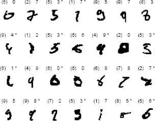
The 28 misclassified digits by the most accurate Network3-ensemble-5 and DropConnect-ensemble-5 are shown respectively in Figure 4.2.5 and 4.2.5. As it can be observed from these Figures, the misclassified examples are hard to be correctly classified by humans. Moreover, although the two ensembles provide the same accuracy, 99,72%, they classify different difficult instances with different results, i.e., only 13 common instances belong to the two misclassified sets. This interesting result demonstrates the high potential of data-preprocessing to improve the current top-1 accuracy.
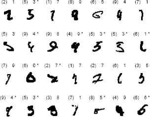
The 28 handwritten digits misclassified by ensemble-5 of Network3 trained during 10 epochs. The digit between () represents the correct class. The 13 digits labeled with asterisks are also misclassified by DropConnect based ensemble-5.
The 28 handwritten digits misclassified by ensemble-5 of DropConnect trained during 10 epochs. The digit between () represents the correct class. The 13 digits labeled with asterisks are also misclassified by Networks based ensemble-5.
4.3. Execution time
All the experiments have been carried out on an Intel(R) Core(TM) i7-3770K CPU connected to Nvidia GeForce GTX TITAN GPU (see its characteristics in Table 13). The bandwidth between host and device, measured using Nvidia bandwidthT-est benchrmak, is 6641.1 MB/s. For the experiments in Theano we have used optimization flags THEANO⎽FLAGS=’floatX=float32,device=gpu0,lib.cnmem=1,optimizer⎽including=cudnn’.
| Global memory | 6 GB |
| # of multiprocessors | 14 |
| # of cores/multiprocessor | 192 |
| CUDA version | 7.5 |
Characteristics of the GPU used in the experiments.
We have also reported the execution time of the most computationally expensive process in deep learning, which is the training phase, in columns 5 and 9 in Table 7 and columns 4 and 7 in Tables 8 and 9. As we can observe, the execution time of LeNet and DropConnet is not affected by the size of the training datasets. That is, training LeNet and DropConnect on the transformed datasets take the same duration as training them on the original set. This is because they analyze the same number of examples independently on the size of the training set. However, the execution time of Network3 is higher on larger datasets. This is due to the differences in how the stop criteria are implemented in each code/library, e.g., Caffe stop criteria is based on the number of iterations.
5. Conclusions
We have presented a short description of image preprocessing for deep learning algorithms in general and CNNs in particular. We have analyzed the impact of different preprocessing techniques, configu-rations and ensembles on the performance of three networks, LeNet, Network3 and DropConnect. The latter represents the current state-of-the art. We used the problem of handwritten digits recognition as case of study and evaluated individual and combinations of the considered preprocessing methods on the MNIST dataset.
Our results demonstrate that the combination of elastic and rotation improves the accuracy of the three analyzed networks up to 0.71%. Ensembles together with preprocessing improve the accuracy, with respect to the original non-preprocessed models, up to 0.74%. A remarkable result is that different high performing ensembles misclassify different examples, which evidences that there is still room for further improvement. As future work, we will focus on improving the state-of-the art accuracy in MNIST classification.
Acknowledgments
This work was partially supported by the Spanish Ministry of Science and Technology under the project TIN2014-524 57251-P and the Andalusian Research Plans P11-TIC-7765. Siham Tabik was supported by the Ramon y Cajal Programme (RYC-2015-18136).
References
Cite this article
TY  - JOUR
AU  - Siham Tabik
AU  - Daniel Peralta
AU  - Andrés Herrera-Poyatos
AU  - Francisco Herrera
PY  - 2017
DA  - 2017/01/01
TI  - A snapshot of image pre-processing for convolutional neural networks: case study of MNIST
JO  - International Journal of Computational Intelligence Systems
SP  - 555
EP  - 568
VL  - 10
IS  - 1
SN  - 1875-6883
UR  - https://doi.org/10.2991/ijcis.2017.10.1.38
DO  - 10.2991/ijcis.2017.10.1.38
ID  - Tabik2017
ER  -