
Size and Location Diagnosis of Rolling Bearing Faults: An Approach of Kernel Principal Component Analysis and Deep Belief Network
 , Sibo Yu1, Weijie Gu1
- DOI
- 10.2991/ijcis.d.210518.002How to use a DOI?
- Keywords
- Rolling bearings; Fault diagnosis; Incipient faults; Kernel principal component analysis; Deep belief network
- Abstract
Diagnosing incipient faults of rotating machines is very important for reducing economic losses and avoiding accidents caused by faults. However, diagnoses of locations and sizes of incipient faults are very difficult in a noisy background. In this paper, we propose a fault diagnosis method that combines kernel principal component analysis (KPCA) and deep belief network (DBN) to detect sizes and locations of incipient faults on rolling bearings. Effective information of raw vibration signals processed by KPCA method is used as input signals of the DBN of which weights of the first RBM are initialized by contribution rates of principal components. A DBN with complex structures can be cut into a briefer network by KPCA-DBN model. That model reduces network structure and increases convergence rate. As a result, an average test accuracy by KPCA-DBN can reach 99.1% for identification of 12 labels including incipient faults and the training time is 28s which is half of that by DBN model. The average accuracy of rolling bearing location detection nearly gets to 100% and the average accuracy of fault size detection is above 99%. Compared with SVM, BP, CNN, Deep EMD-PCA (Empirical Mode Decomposition-Principal Component Analysis), CNN-SVM and DBN, it is found that training time can be shortened and detection accuracy can be improved by KPCA-DBN model. The proposed method is beneficial to realize sizes and locations detection of incipient faults online.
- Copyright
- © 2021 The Authors. Published by Atlantis Press B.V.
- Open Access
- This is an open access article distributed under the CC BY-NC 4.0 license (http://creativecommons.org/licenses/by-nc/4.0/).
1. INTRODUCTION
The vibration signal of incipient fault [1] belongs to weak signals with low signal to noise ratio (SNR). The dynamic characteristics generated by incipient faults are usually submerged in noise signals. Hereby, it is a focused problem to accurately identifying the incipient faults mixed with serious faults and normal signals in a noisy background. If incipient faults are failed to detect, opportunity for maintenance may be missed leading to a serious fault.
In recent years, with research on artificial intelligence (AI), the intelligent algorithms [2] were applied to fault diagnosis of rolling bearings. Features can be automatically extracted by wavelet transform (WT) [3], spectral analysis (SA) [4], etc. A relationship between features and states was established based on machine learning [5] or neural network for diagnose faults. Although these methods [6–8] can classify machine faults, there are still some disadvantages as follows: (1) The fault diagnosis results are depended on massive raw data. For example, a novel method [9] combining the Z-number and Dempster–Shafer (D-S) evidence theory was proposed to provide reliable information from massive sensor data for fault diagnosis. The intelligent methods [10] of machine learning and shallow neural network [11] are limited in learning so they depend on enough information to extract representative features and be trained fully. (2) A multi-step (feature extraction, feature selection and training classifier) process of fault diagnosis reduced efficiency. Normally, those methods need to extract time-domain, frequency-domain and time-frequency-domain features [12] of vibration signals. Furthermore, a feature selection technique was employed to obtain a feature subset and a cost-sensitive learning method was designed for a classifier. All the processes actually weakened overall efficiency of the methods. (3) Feature selection brings about the interference of human factors. Canfei et al. [13] adopted two criteria for measuring diagnostic performance which were assessed by sparse Bayesian extreme learning machine (SBELM). Further, F-measure was adopted to identify the optimal feature subset. As a result, some useful information may have been filtered by human factors. (4) Representative features are only retained but incipient fault features are easily ignored [10]. As an incipient fault is not distinct, it may be missed in feature selection or noise reduction.
In view of those problems above, deep learning [14–16] was proposed by Hinton, et al, which no longer relied on manual feature selection. Deep learning can directly extracted features from raw data automatically [17] and showed great intelligence and effectiveness in fault diagnosis. Yu et al. [18] proved that features inherent in raw temporal signals were extracted hierarchically and automatically by stacking LSTM, which can achieve up to 99% accuracy for fault diagnosis of rolling bearings. A new roller bearing fault diagnosis algorithm was presented based on a sparsity and neighborhood preserving deep extreme learning machine (SNP-DELM) [19], by which deep features were extracted layer by layer without supervision. A model of CNN with less learnable parameters was proposed by Verstraete [20], which achieved better diagnosis accuracy on fault diagnosis of rolling element bearings. A method was presented of denoising stacked auto-encoder (DSAE) in deep learning without principal components analysis [21]. Recently, a novel adaptive Fisher-based deep convolutional neural network (AFDCNN) [22] method was proposed which was an improvement of the FDCNN and used to diagnose faults of small samples.
Furthermore, deep belief network (DBN) which is one of deep learning is widely adopted in fault diagnosis for its classification capability of multiple types [23,24]. Compared with feed-forward multi-layer perceptron neural network, Dedinec et al. [25] provided superior calculation results by DBN in hourly electricity load forecasting of the Macedonian electric power system. An enhanced intelligent fault diagnosis method was proposed based on pairwise graph regularized deep belief network (PG-DBN) model [26], which got a better classification result of fault diagnosis. A framework of SOM-DBN was applied to fault early warning system for dispatching automation [27]. Feature vectors which were fused by sparse autoencoder (SAE) neural networks were used to train a DBN to distinguish faults. Tran et al. [28] indicated statistical features were extracted from all signals to represent the characteristics in conditions and a DBNs was built to classify faults of compressor valves. A novel method called adaptive DBN with dual-tree complex wavelet packet (DTCWPT) was developed [29] to improve identification accuracy. There are also a lot of other successful applications in fault diagnosis of rotating machinery [30,31] based on DBN. Researches show that DBN has good characteristics in automatic feature extraction and multi-task classification. However, they all built a multi-layer DBN structure for feature learning and extraction, which would lead a long time duration for training and testing. For rapid worsening incipient faults, fault features change from time to time. If it takes long time to train and test a DBN model, it would have a negative impact on real-time detection of incipient faults. In addition, they did not focus on the location identification of incipient faults in a noisy background by DBN.
We focus on sizes and locations diagnosis of incipient faults, which can help to reduce work of faults checking and maintenance. In this paper, we propose a method of kernel principal component analysis (KPCA)-DBN to diagnose incipient faults rapidly and accurately without artificial features extraction and selection. For the proposed method, effective information of raw data is kept by KPCA [32,33] instead of feature statistics and feature extraction without destroying structures and distributions of raw data. The method of KPCA-DBN can simplify the network structure of DBN and adjust initial values of weights, which improves convergence speed and diagnosis accuracy. Diagnosis accuracy can be increased and training time can be shortened by KPCA-DBN, which solves the problem of real-time detection of incipient fault. Furthermore, the diagnosis results by the method of KPCA-DBN for fault diagnosis of 12 failure types including incipient faults are compared with those by the common methods which involves SVM, BP, KNN [34], Deep EMD-PCA [5], CNN-SVM [35] and DBN. Diagnosis results show that KPCA-DBN model is more effective than the other methods mentioned in both efficiency and accuracy.
Besides, noise is an important factor for identification of incipient faults. Wavelet threshold denoising [36] is one of common denoising measures and it has been limited for lacking of adaptive decomposition [37]. In view of the problem, variational modal decomposition (VMD) [38] was presented.
In this paper, we propose a denoising method of VMD-Sample entropy–wavelet threshold denoising to process raw data for enhance signal noise ratio of vibration signals without losing incipient fault features of rolling bearing. Then we use KPCA-DBN model to diagnose incipient faults. In a noisy background, this method can also reduce training time for identifying different sizes and locations of the incipient faults even mixed with multiple failures.
2. BRIEF REVIEW OF KPCA-DBN
2.1. Kernel Principal Component Analysis
KPCA method can map input data to high-dimensional space by nonlinear kernel functions. The data linearly indivisible in original sample space can be separated in feature space and nonlinear principal components [39] are separated.
X is a sample space and H is a characteristic space (Hilbert space). If map X to Η by
Given a kernel function for a training set S.
A covariance matrix in high-dimensional space and kernel matrix.
The covariance matrix CF of the mapping matrix
where F represents high-dimensional feature space, λ is the eigenvalue, V is the eigenvector, M represents dimension of original data.The projection of an eigenvector by mapping data in original space is expressed by Eq. (3).
whereEq. (3) is carried out on the premise of assuming that the average value of mapped data is equal to zero [40], so it is necessary to realize centralization of mapped data by K replaced by
where LM is a matrix ofThe nonlinear principal components
2.2. Deep Belief Network
DBN is regarded as a multi-layer perceptron neural networks composed of restricted Boltzmann machines (RBMs) [41,42] in the first stage. In Figure 1, each RBM consists of a visible layer (v) and a hidden layer (h).
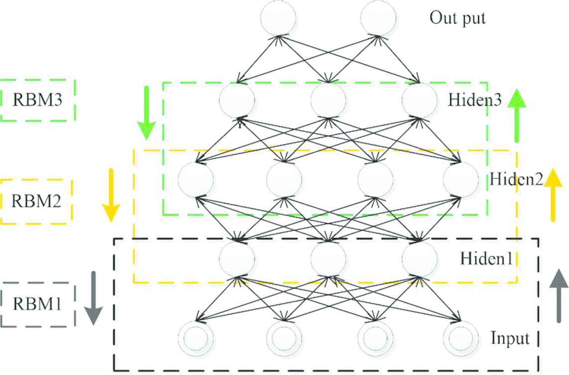
DBN structure with three hidden layers.
Greedy learning is an unsupervised training process. Second stage [44] is to regard the tag layer as the top layer and conduct supervised fine-tuning from the top to the bottom.
Energy model is adopted as a measure of system in the steady-state. The process of training RBM is constantly to change the scalar energy. Energy function E is defined as Eq. (6).
Joint probability distribution of states
Conditional probability distribution is expressed by Eqs. (10) and (11).
The purpose of training RBM structure is to meet the distribution of training data. Calculating the maximum likelihood estimation of parameter θ is shown as Eqs. (12) and (13).
A method of contrastive divergence (CD) [14] is proposed by Hinton to speed up the calculation of the log-likelihood gradient to solve the problem of low calculation efficiency.
Step 1: Set network structure and initialize parameters.
Step 2: Training.
A training sample
Update weights and offsets.
Update of parameters by Eqs. (14–18).
Step 3: The labels are attached to the top layer to fine tune with a back-propagation algorithm.
In fact, there is an error between outputs of model and labels. When the output layer of DBN is regarded as the first layer of back-propagation neural network, the error will be propagated from the top layer down to each layer of RBM for fining tune the whole DBN. Obviously, fine-tuning is a supervised training process in the second stage, which is different from the unsupervised self-learning process in the first stage. It can be seen that DBN is a deep model with feature learning and classification by the two-stage training.
3. GENERAL PROCEDURES OF BUILDING A MODEL FOR BEARING FAULT DIAGNOSIS
The general procedures of the proposed method are summarized as Figure 2.
Step 1: Bearing vibration signals are decomposed by VMD. Sample entropy of IMFs is sorted from large to small and the first two IMFs are selected to be processed by wavelet threshold denoising.
Step 2: Reconstructed signals after denoising are processed by Hilbert transform and by FFT.
Step 3: Choose kernel function and dimensions of raw data set. The raw data is dimensioned by KPCA to form input data into DBN.
Step 4: Structure a DBN for diagnosis.
Step 5: Further improve accuracy and training speed by optimizing the network parameters. Specifically weight matrix of DBN is initialed by a contribution rate of principal components and key parameters of KPCA-DBN are adjusted.
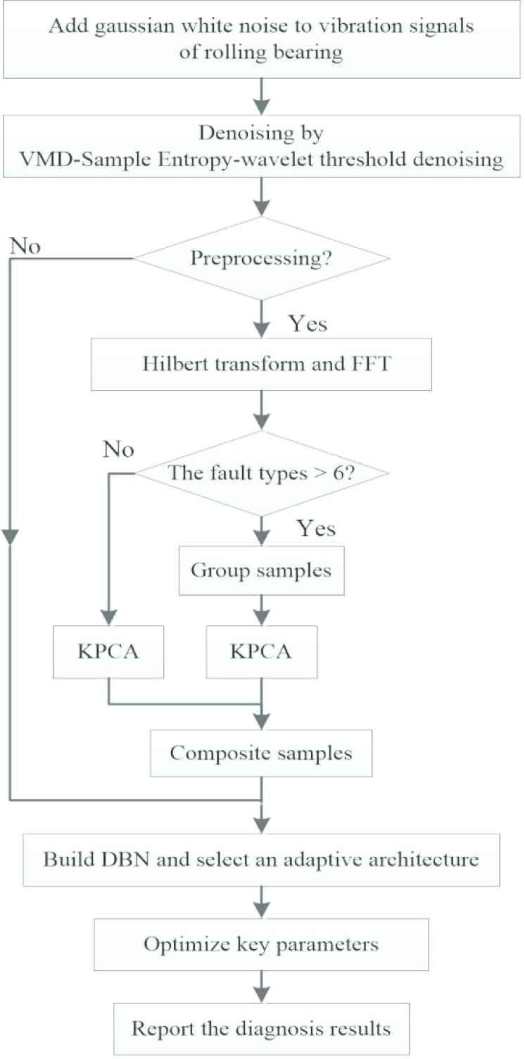
The flow chart of diagnosis model by proposed method.
4. EXPERIMENTAL DATA DESCRIPTION
The vibration signals of rolling bearing are from experimental data of Case Western Reserve University [45]. The test bench consists of a 2hp three-phase induction motor shaft and a dynamometer for generating rated load in Figure 3. The vibration signals of drive end bearing are generated at a 1750 rpm motor speed. The sampling frequency fr is 12 kHz. All vibration signals have 12 states in total, which are labeled from 1 to 12. Some labeled states are combined to form different categories (ClassX or ClassX-X) with different fault locations and sizes. Class1 is for distinguish four faults on different positions of a rolling bearing. Class2 is for distinguish different fault sizes at a same location of rolling bearings. Fault states can be subdivided into three groups, Class2-1, Class2-2 and Class2-3, depending on different positions of rolling bearing. Class3 is for distinguish different locations of faults on outer race with different angles relative to the load zone. The last category marked by “All class” represents a data set containing all 12 labels. Each faults contain 115 samples and each sample consists of 1024 data points. All the labels are shown in Table 1.
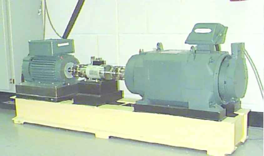
Experimental device.
| Bearing Position | Fault Diameter (in) | Fault Placement | Label | Category |
|---|---|---|---|---|
| Normal | 0 | 0 | 1 | Class1 (Class1) |
| Inner race faults | 0.007 | 0 | 2 | Class2-2 (Class1) |
| 0.014 | 3 | Class2-2 | ||
| 0.021 | 4 | Class2-2 | ||
| Ball faults | 0.007 | 0 | 5 | Class2-3 (Class1) |
| 0.014 | 6 | Class2-3 | ||
| 0.021 | 7 | Class2-3 | ||
| Outer race faults | 0.007 | @3:00 | 8 | Class3 (Class1) |
| @6:00 | 9 | Class3 (Class2-1) | ||
| @12:00 | 10 | Class3 | ||
| 0.014 | @6:00 | 11 | Class2-1 | |
| 0.021 | @6:00 | 12 | Class2-1 |
Classification description of case western reserve bearing [45].
5. RESULTS AND ANALYSIS
5.1. VMD and Wavelet Threshold Denoising
The average SNR of all signals is 5 when signals are added strong noise, and the SNRs of signals with label 1, 2, 8, 9 and 10 are negative. That means signal power is less than noise power. In addition, signals with label 2, 8, 9 and 10 is the vibration signals which crack diameter of rolling bearings are only 0.007 in and the fault features are easy to be submerged in noise so they are considered as incipient faults.
Each sample of above signals is decomposed into 5 IMFs by VMD. The sample entropy of IMFs is calculated and listed in descending order. Then the first two IMFs are selected to be processed by wavelet threshold denoising to reduce noise and prevent incipient fault features from being filtered. Select “db3” wavelet function and choose the number of wavelet decomposition layers to be 4. Noise is concentrated in a high-frequency coefficient and that part is filtered out in a reconstructed signal through an appropriate threshold. Finally, noise is suppressed.
Denoising performance is evaluated by SNR and root mean square error (RMSE). At first, 75000 sampling points of signals with label 2 are taken for experiment and the SNR is −0.85. The theoretical failure frequency of the fault on inner race is 159.4 Hz [46]. It can be seen from Figure 4(b) that the amplitude of failure frequency is too small to identify in IMF1. Besides, failure frequency is easily confused with a several peaks in the neighborhood of the frequency in IMF5. However, the tagged frequency of 158.2 Hz in IMF1 and IMF5 can be clearly identified when signals are processed by the proposed noise-reducing method in Figure 4(c). A tagged frequency is almost equal to 159.4 Hz and they are considered to be consistent. In addition, the fault feature is more obvious by denoising. SNR is increased from −0.85 to 6.6 by denoising.
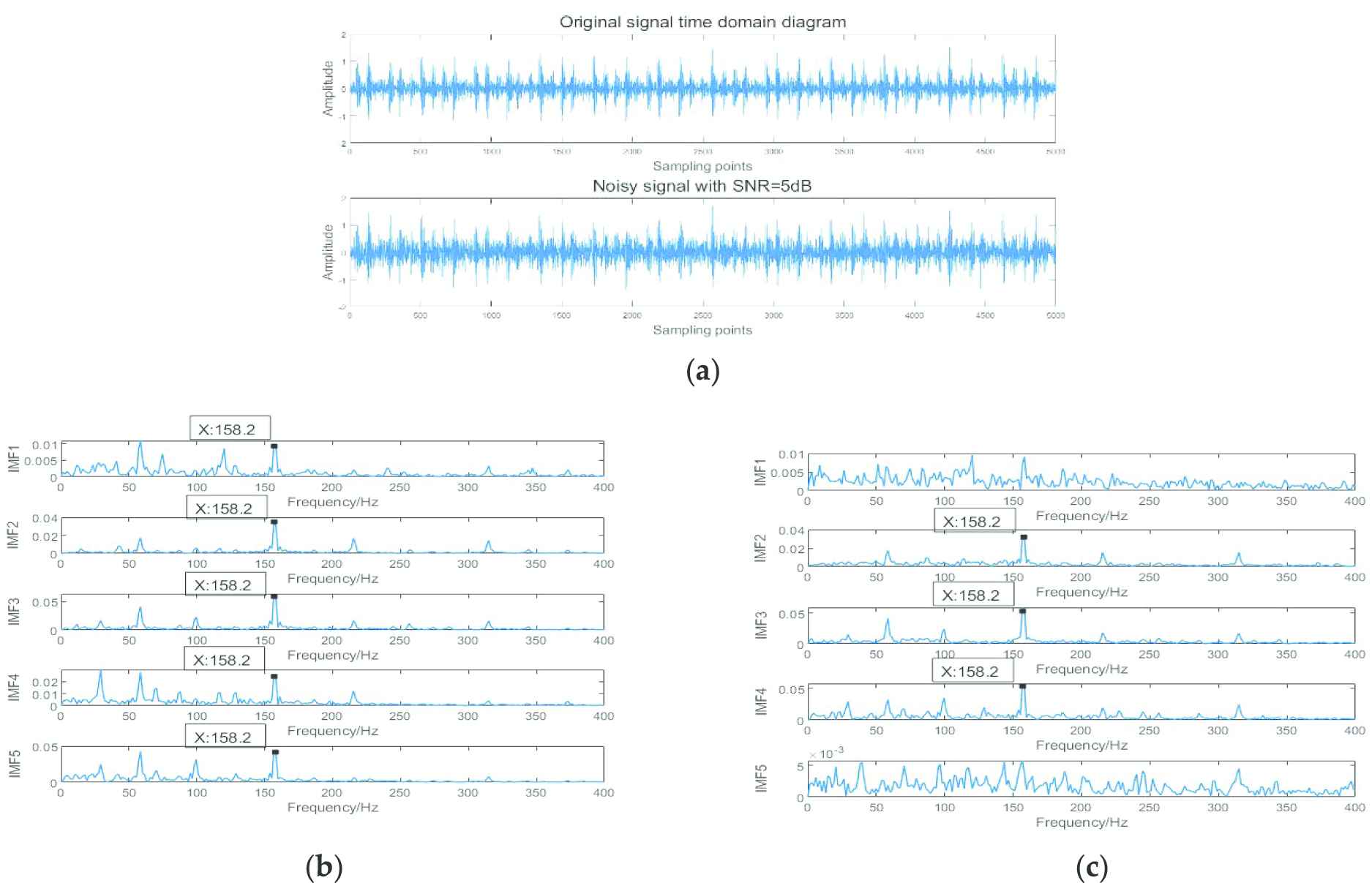
Vibration signals and corresponding spectrum of noisy IMFs and denoised IMFs. (a) Measured vibration signal and the signal added noise; (b) spectrum of IMFs decomposed from signal added noise; and (c) spectrum of IMFs decomposed from denoising signal.
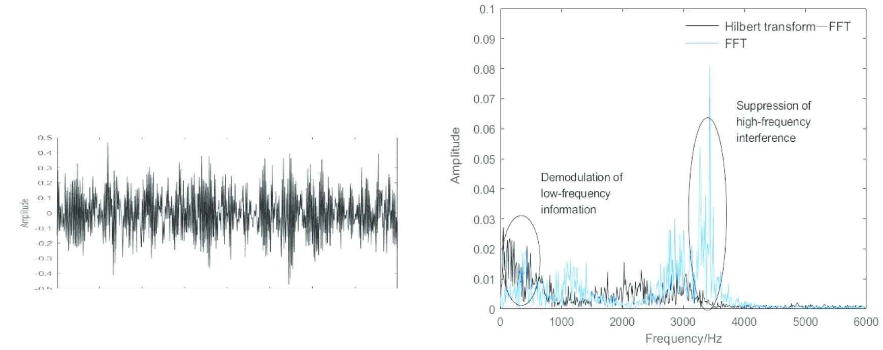
Hilbert transformation and Fourier transform. (a) Denoised vibration signal and (b) spectrum of preprocessed signal by Hilbert transformation and FFT and Spectrum of preprocessed signal by FFT.
Secondly, denoising results of signals with “Class3” by different methods are compared in Table 2. It shows that the performance by VMD-sample entropy–wavelet threshold denoising is superior to others.
| Methods | Evaluation Indicator | Class3 |
||
|---|---|---|---|---|
| 8 | 9 | 10 | ||
| Measured vibration signals added with noise | SNR | −0.16 | −0.41 | −2.92 |
| RMSE | 0.0502 | 0.0502 | 0.0504 | |
| VMD | SNR | 3.59 | 3.44 | 0.94 |
| RMSE | 0.0325 | 0.0323 | 0.0422 | |
| Wavelet threshold denoising | SNR | 0.23 | 0.17 | 0.11 |
| RMSE | 0.0441 | 0.0467 | 0.0475 | |
| VMD-sample entropy-wavelet threshold denoising | SNR | 6.80 | 7.20 | 5.07 |
| RMSE | 0.0281 | 0.0268 | 0.0293 | |
Denoising effect of signals with “Class3.”
If wavelet threshold denoising is applied to each IMF by VMD-wavelet threshold denoising, most noise will be eliminated but some useful information including incipient fault features may be lost. We use signals of “Class3” to test useful information lost. The measured vibration signals added with noise and the signals denoising by the following two methods are input into DBN to obtain the fault diagnosis results for comparisons. Mean accurate rates of diagnosis are shown in Table 3. Network structure of DBN has three hidden layers and the number of hidden layer nodes is set as [500, 300, 100]. Learning rate is 0.001 and iteration number is 1000. Each experiment is calculated 10 times.
| Methods | Fault Diagnosis Times | Average Accuracy |
|---|---|---|
| Measured vibration signals added with noise | 10 | 31% |
| VMD-sample entropy-wavelet threshold denoising | 10 | 48% |
| VMD-wavelet threshold denoising | 10 | 38% |
Effect of denoising methods on diagnosis results.
From Table 3, the proposed noise-reduction method is effective to filter strong noise of vibration signals of incipient faults and helpful to improve diagnosis accuracy.
5.2. The Proposed Method of KPCA-DBN
Fault features in time-domain are difficult to be recognized effectively, by which diagnosis results of DBN show low classification accuracy in Table 3. However, the fault diagnosis results [27] by DBN for frequency-domain signals have been improved significantly. In this paper, the denoised vibration signal is transformed into an analytical signal by Hilbert transformation and then converted to a frequency-domain signal by fast Fourier transform (FFT). In addition, richer information in low frequency and less interference in high frequency of frequency-domain are shown by Hilbert transform-FFT in compared with that only transformed by FFT when processing the data of label 9.
The data set from “All class” involving 12 labels is preprocessed to reduce dimension from 1024 to 513. Two methods of traditional DBN and KPCA-DBN are adopted to classify 12 labels. For the method of KPCA-DBN, data set firstly is divided into 2 categories and each category contains only 6 faults because the KPCA method is an unsupervised dimensional reduction method which determines the limitations in dealing with multi-label data. KPCA algorithm is applied to reduce dimension for each category and then combine them into a matrix as input data of DBN. The number of principal components retained by KPCA is set as 300, then training set is an 870 × 300 matrix and test set is a 345 × 300 matrix. For the method of traditional DBN, the data dimension keeps to 513 so the data set is divided into an 870 × 513 matrix for training and a 345 × 513 matrix for testing. Data dimension will determine the number of nodes in visible layer of the first RBM in DBN. Structure of DBN is very important for feature extraction and states recognition. In this paper, DBN has three hidden layers and the number of hidden layer nodes is set as [500, 300, 100]. Learning efficiency is 0.001 and the number of iterations is 1000. Average accuracy and average training times are calculated for ten test to ensure reliability. In comparison, DBN is designed to has two hidden layers and the number of hidden layers nodes are respectively [300, 100] and [100, 50] without changing network parameters and data form. Average accuracy and training time by traditional DBN and KPCA-DBN for “All class” are shown in Table 4.
| Hidden Layer Nodes | Methods | Input Layer Nodes | Output Layer Nodes | Average Test Accuracy (%) | Average Training Time (s) |
|---|---|---|---|---|---|
| 500-300-100 | DBN | 513 | 12 | 96.5 | 151 |
| KPCA-DBN | 300 | 12 | 87.4 | 104 | |
| 300-100 | DBN | 513 | 12 | 95.3 | 57 |
| KPCA-DBN | 300 | 12 | 94.1 | 35 | |
| 100-50 | DBN | 513 | 12 | 95.1 | 42 |
| KPCA-DBN | 300 | 12 | 94.6 | 21 |
Average accuracy and training time by traditional DBN and KPCA-DBN for “All class.”
In Table 4, the test accuracy obtained by KPCA-DBN increases significantly when reducing the number of hidden layers of DBN. It indicates that overfitting may occur when hidden layers is three. It shows that the test accuracy by the KPCA-DBN which DBN has two hidden layers is close to that by traditional DBN which has three hidden layers but the training time is only one fifth (35/151) of that taken by traditional DBN in Table 4. With decreasing the number of nodes of two hidden layers, the network is simplified further and the classification accuracy by KPCA-DBN is increased slightly from 94.1% to 94.6%. It shows that the proposed method of KPCA-DBN can simplify network and shorten training time to 21s meanwhile it still reaches above 94% diagnosis accuracy for multiple faults including incipient faults.
5.2.1. Analysis of kernel function
The recognition accuracy by the proposed method isn't getting enough accurate as it is mainly limited in DBN structure and settings of KPCA. KPCA maps samples from low- dimensional space to high one. The mapping function
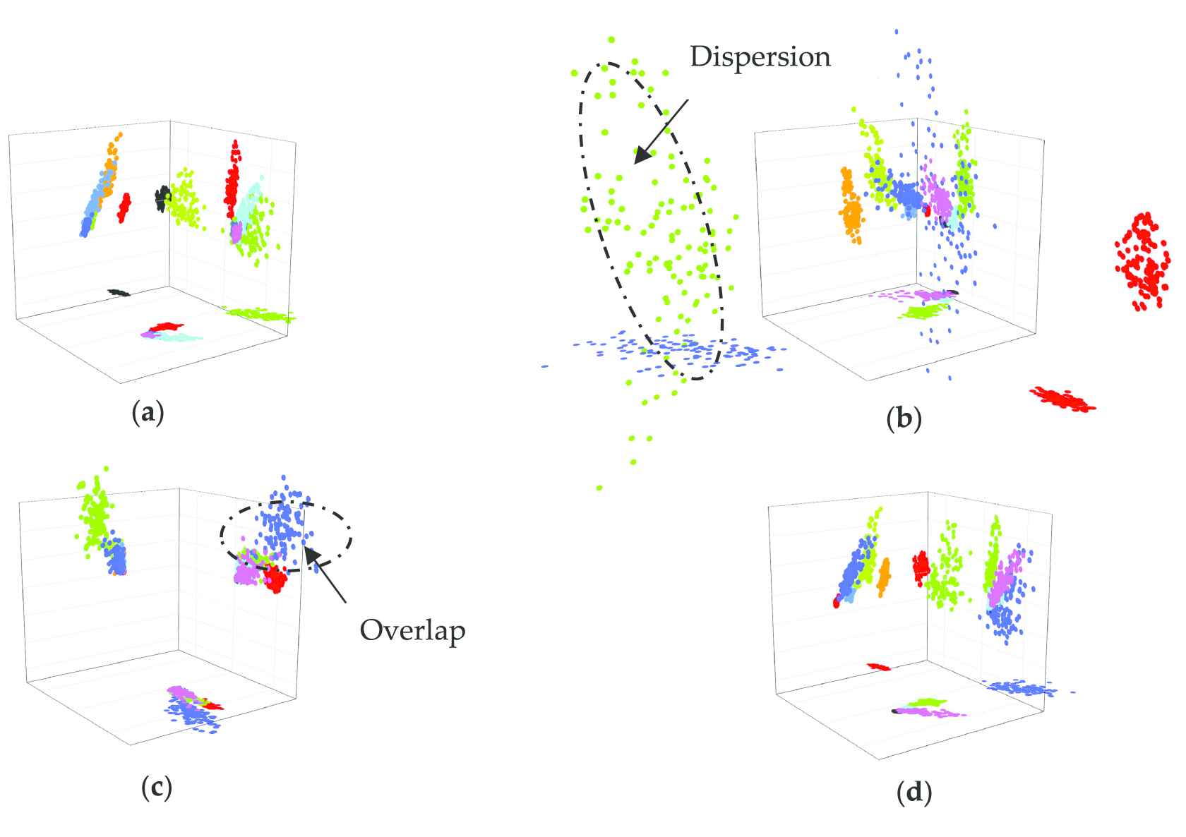
Projection of the first three principal components (
The top three principal components show good performance of clustering in space by both Gaussian kernel function and linear kernel function. However, clustering by Polynomial Kernel is not ideal. The clustering points of label 2 and 4 are scattered that the principal components extracted from different samples with the same label by Polynomial Kernel are distributed or scattered in some different directions in the space. Oppositely the principal component can basically cluster by Laplacian Kernel function but centers of clustering in different colors are heavily overlapped so that different labels cannot be separated. The overlapping shows that different features of multi-label samples are hard to characterize by Laplacian Kernel function. Compared with Gaussian kernel function, the distance between the clustering centers of different labels is smaller than that by linear kernel function so linear kernel function is selected. It follows then that a suitable kernel function is beneficial to linear separability of multi-label data in feature space.
5.2.2. Analysis of the number of principal components
The process of forming input samples by KPCA not only determines dimension of input sample but also the validity of data information. The number of principal components is set as 300, 200, 100, 10 and 5 so input matrix with different dimensions are formed to input into DBN. DBN is constructed with two hidden layers and nodes of hidden layers is [100, 50]. Units of output layer in DBN are adjusted to meet data of different fault types shown in Table 5. Learning rate is 0.001, iterations is 1000 and loss detection period is 10. Each experiment is repeated 10 times and the average accuracy and training time are recorded.
| Structure of DBN | Class1 | Class2-1 | Class2-2 | Class2-3 | Class3 | All Class |
|---|---|---|---|---|---|---|
| Units of output layer | 4 | 3 | 3 | 3 | 3 | 12 |
Description of output data size.
Average training time is shown by bar graph and average accuracy of different categories is plotted in Figure 7 by calculation of 10 times. With decrease of number of principal components, dimensions of input matrix in DBN is getting small and training time is shortened. When the number of principal components reduces from 300 to 100, the training times for “All class” are 19.2s, 15.7s, 8.9s in order and average accuracy increase from 94.9% to 96.7%. Therefore, the computing time can be reduced without decreasing accuracy if the principal components kept from measured data are enable to cover the primary features. When the number of principal components is reduced to only 2% of dimensions of measured data, average accuracies of all classification are plotted in gray line and the values of points are 98.8%, 98.8%, 96.6%, 97.6%, 98.6% and 93.1%. Compared with results of 100 dimensions, average accuracy has reduced. The decline of average accuracy is very obvious when the principal components are only 1% of dimensions of measured data. Take “All class,” e.g., whose average accuracy has dropped to 90.72%. Seen from the average accuracies, the principal components which rank the top 20% of the eigenvalue contribution rate have represented sensitive features of measured data and redundant interference features can be removed by KPCA. However, when principal components are kept a little, too much data filtered will lose a lot of information and decreases accuracy. As a result, it is reasonable to generate input sample with 100 dimensions by KPCA in this paper.
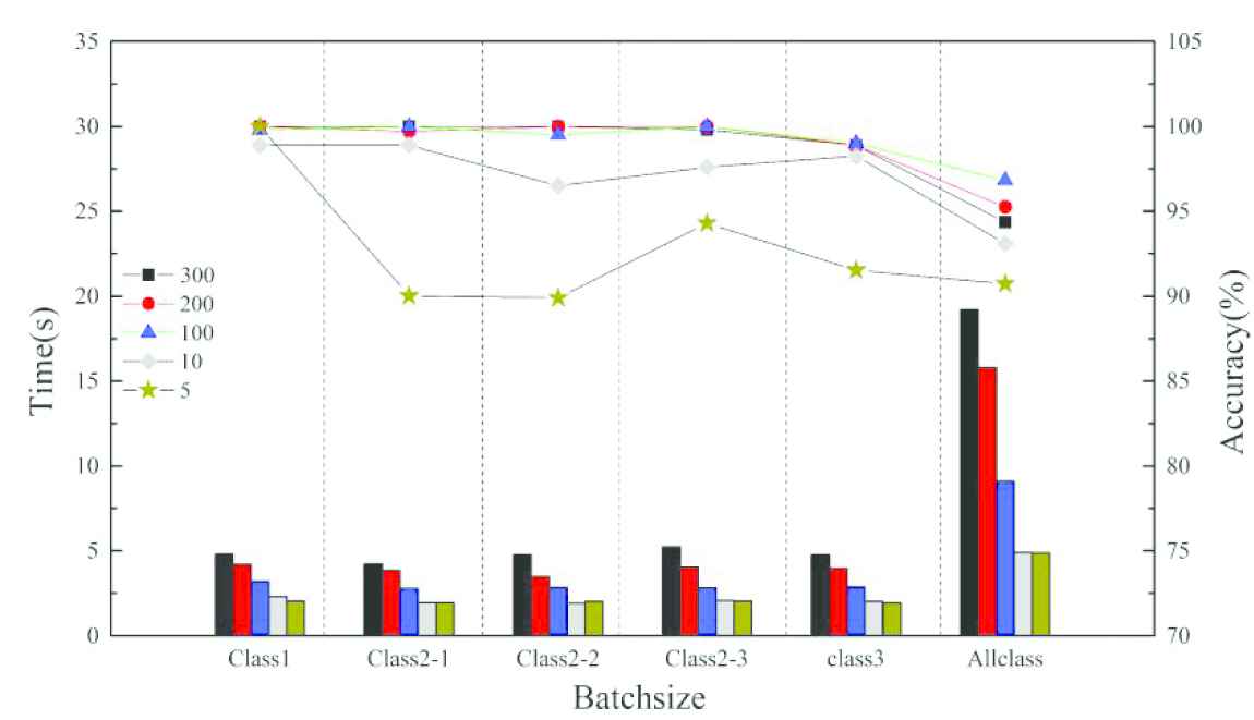
Average accuracy and training time with different number of principal components.
5.3. Comparison with Other Methods
We will compare KPCA-DBN method to other intelligent methods by the same fault data shown in Table 6. BP, SVM, KNN, CNN-SVM, Deep EMD-PCA and DBN are compared. 85 samples are randomly selected from each category to train and the rest 30 samples for testing.
| Methods | Class1 |
Class2-1 |
Class2-2 |
Class2-3 |
Class3 |
All Class |
||||||
|---|---|---|---|---|---|---|---|---|---|---|---|---|
| A (%) | T (s) | A (%) | T (s) | A (%) | T (s) | A (%) | T (s) | A (%) | T (s) | A (%) | T (s) | |
| BP | 78.3 | 3.1 | 79.6 | 3.5 | 81.7 | 2.8 | 79.4 | 3.6 | 76.1 | 4.3 | 78.9 | 8.7 |
| SVM | 82.8 | 2.9 | 86.8 | 3.1 | 85.8 | 2.2 | 86.2 | 2.1 | 81.1 | 3.3 | 83.7 | 8.2 |
| KNN | 91.4 | 10.3 | 87.3 | 9.9 | 89.1 | 9.7 | 88.1 | 10.4 | 87.4 | 9.8 | 84.1 | 54.7 |
| CNN-SVM | 100 | 16.8 | 100 | 16.3 | 99.8 | 15.9 | 100 | 17.2 | 99.7 | 16.9 | 99.4 | 73.8 |
| Deep EMD-PCA | 88.6 | 25.6 | 86.2 | 25.3 | 86.9 | 24.3 | 87.5 | 25.5 | 87.9 | 25.8 | 84.8 | 142.1 |
| DBN | 98.3 | 9.2 | 99.6 | 7.2 | 99.1 | 7.7 | 98.1 | 8.4 | 97.4 | 8.9 | 95.1 | 42 |
| KPCA-DBN | 98.8 | 4.2 | 99.4 | 3.7 | 99.3 | 3.5 | 98.9 | 3.9 | 98.2 | 4.6 | 95.3 | 9.3 |
Average accuracy and training time of four different methods data.
Results of fault diagnosis by SVM, BP and KNN are based on training the statistical features. 14 statistical features of each bearing fault sample are calculated by the method in the literature [47] and the detailed parameters are listed in Table 7. Then, the 14 statistical features are input into BP, SVM and KNN for fault diagnosis. BP neural network has a one hidden layer with 100 nodes. For the method of Deep EMD-PCA, principal space and residual space of dataset are decomposed two times to obtain the 4-layer subspace by EMD. Then, constitute input matrix by IMFs decomposed from EMD, which is input data of PCA to cluster different fault types. When using CNN-SVM method to diagnose faults the details about the structure of CNN are shown in Table 8. We also use traditional DBN for comparisons. DBN has three hidden layers and the number of hidden layer nodes is [100, 100, 50]. Other parameters of DBN are same as that of KPCA-DBN. The number of principal components of KPCA-DBN is 100. Hidden layer of this model is decrease to be 1 and the nodes of the hidden layer are 50. Units of output layer are set according to the number of fault types involved in different data categories. Diagnosis results by seven methods are shown in Table 6.
| Domain | Feature Parameters | |
|---|---|---|
| Time-domain | Absolute mean: |
Root mean square: |
| Variance: |
Shape factor: |
|
| Crest: |
Clearence factor: |
|
| Kurtosis: |
Pulse factor: |
|
| Skewness: |
Crest factor: |
|
| Frequency-domain | Crest: |
Variance: |
| Kurtosis: |
Mean energy: |
|
14 Statistical features.
| CNN-Softmax Model Structure |
|
|---|---|
| Layer Type | Parameter Settings |
| Input layer | (Batch, 25 × 20, 2) |
| Convolution layer 1 | Filter = (3 × 3, 2, 64), strides = (1, 1), padding = same |
| Activation layer 1 | ReLU activation function |
| Max-pooling layer 1 | ksize = (1, 2 × 2, 1), strides = (2, 2), padding = same |
| Convolution layer 2 | Filter = (3 × 3, 2, 64), strides = (1, 1), padding = same |
| Activation layer 2 | ReLU activation function |
| Max-pooling layer 2 | ksize = (1, 2 × 2, 1), strides = (2, 2), padding = same |
| Convolution layer 3 | Filter = (3 × 3, 2, 64), strides = (1, 1), padding = same |
| Activation layer 3 | ReLU activation function |
| Global average polling layer | ksize = (1, 5 × 4, 1), strides = (5, 4), padding = same |
| Flatten layer | Flatten global average polling layer to 1-D shape |
| FC-Dense layer 1 | 128 hidden layer neuron nodes |
| FC-Active layer 1 | Activation function |
| FC-Dense layer 2 | 12 hidden layer neuron nodes |
| Softmax output layer | Softmax activation function |
The descriptions of the hyper-parameters of CNN.
All classification results are shown in Figure 8(a–f). Accuracy is plotted by a line and training time is shown by a histogram. “A” is average accuracy and “T” is average training time in Table 6.
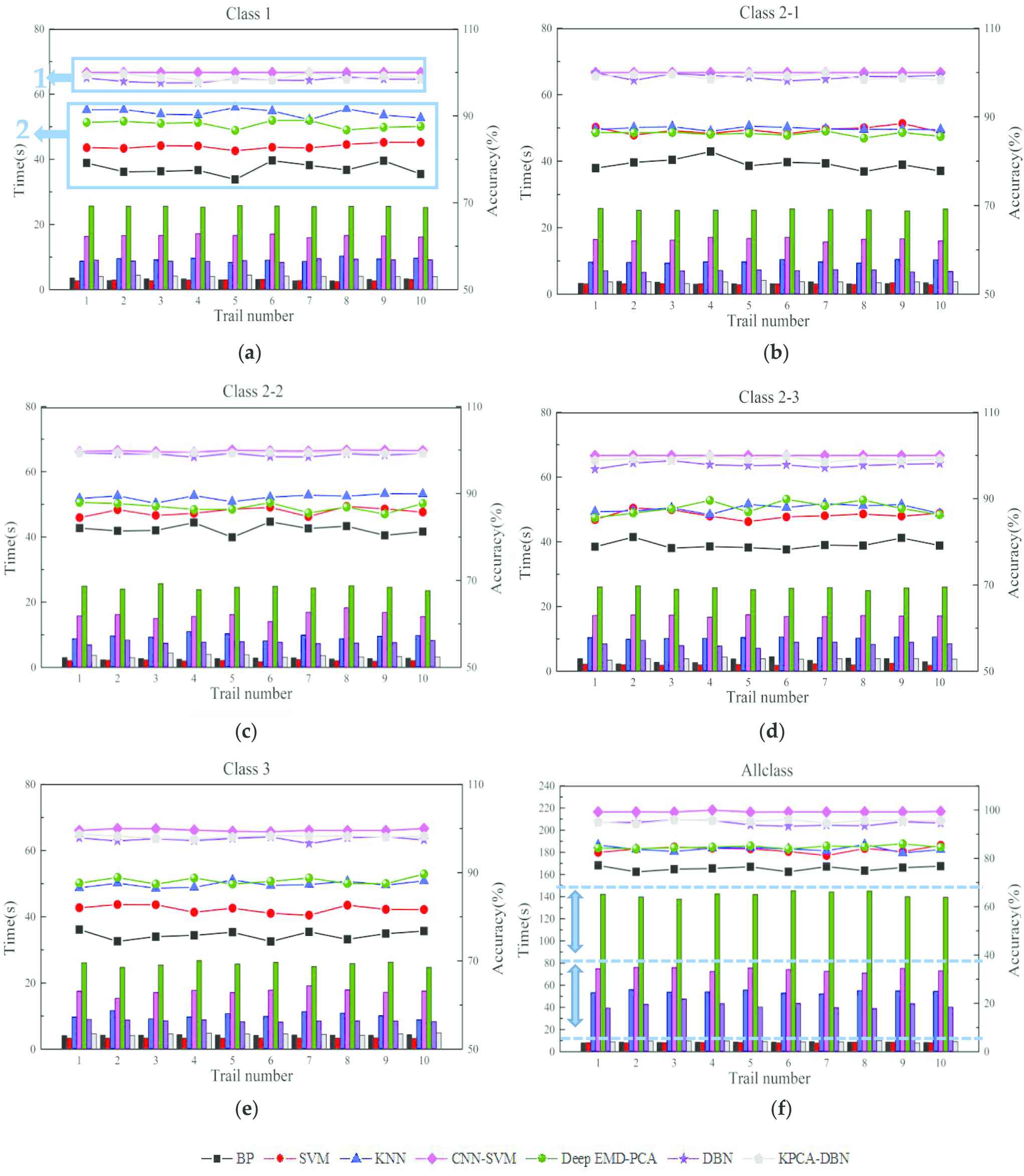
Diagnosis results by four different methods for processing each category data. (a) Class1; (b) Class2-1; (c) Class2-2; (d) Class2-3; (e) Class3; and (f) All class.
Seen from Figure 8, four lines are basically below 90% and other three lines are above 95% and they are divided into regions 1 and 2 in Figure 8(a). Results of CNN-SVM, DBN and KPCA-DBN are in region 1 and results of BP, SVM, KNN and Deep EMD-PCA are concentrated in region 2. The average classification accuracies classified by BP, SVM, KNN and Deep EMD-PCA for “Class3” respectively are 76.1%, 81.1%, 87.4% and 87.9% and the classification accuracy of DBN is improved to nearly 97%. The average accuracy of KPCA-DBN reaches 98.2% and the accuracy of CNN-SVM is the highest even more than 99%. The three methods can distinguish the distribution orientation of incipient faults on rolling bearing. Compared with traditional machine learning and statistic-based algorithms, deep learning network shows a more comprehensive learning performance and is easier to identify the features of vibration signals with low SNRs.
Nevertheless, DBN method takes more than five times as that by SVM (42/8.2) when dealing with data of “All class.” CNN-SVM takes much more time to train which is about 18.5(73.8/42) times than that of DBN, which is the most training time among the three methods in region 2.
It's worth noting that an average diagnosis accuracy of KPCA-DBN for classifying “All class” data reaches 95.3% which is higher than that of DBN. Moreover, KPCA-DBN takes only a quarter (9.3/42) of the training time by DBN and only 13% (9.3/73.8) of the training time by CNN-SVM. That means accuracy diagnosis accuracy of KPCA-DBN is above 95% belonging to region 2 and training time of KPCA-DBN is within 10s closing to that of shallow network. From above, the model of KPCA-DBN gets both high precision and high efficiency.
KPCA-DBN can accurately identify locations and sizes of incipient faults and improve an efficiency of training. It is attributed to that it maps fault data to high-dimensional space when fault data is difficult to be separated in linear space. That overcomes the shortcoming of SVM and EMD-PCA which can only process linearly separable data. Moreover, KPCA algorithm not only preserves the principal components but also eliminates interference of redundant information. The process doesn't depend on the artificial feature selection or feature statistics but an automatic retention for effective information based on data distribution. At the same time, KPCA-DBN model exerts the powerful function of DBN in automatically extracting and learning features. As a result, the proposed method is better than other intelligent algorithms compared with efficiency and accuracy of incipient faults diagnosis. It successfully makes up for the long time-consuming shortcomings of deep learning network (e.g., CNN/DBN).
5.4. Classification Results of KPCA-DBN
5.4.1. DBN structure
Combination of units in hidden layers are divided into stationary, increasing and decreasing type. KPCA-DBN with three different structure types are applied to diagnose faults with data of “All class” shown in Table 9. Each experiment is repeated 10 times and diagnosis results are shown in Figure 9.
| Units per Layer (KPCA-DBN) | Number of Iterations | Training Time | Average Accuracy |
|---|---|---|---|
| 100-50-20-12 (decreasing type) | 1000 | 7.3 | 95.3% |
| 100-100-100-12 (stationary type) | 1000 | 9.8 | 95.4% |
| 100-500-1000-12 (increasing type) | 1000 | 206.5 | 93.9% |
Comparison of DBN structure by KPCA-DBN method.
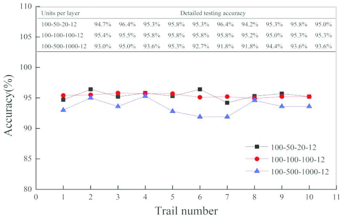
Diagnosis results of KPCA-DBN with different DBN structure.
The accuracy results of decreasing and stationary type are not less 95%. However, the average accuracy of KPCA-DBN with increasing type drops to 93.9% in Table 9. With an increased nodes of layer by layer the classifier is tend to over fitting which will weaken generalization ability of the model. In the view of computational stability, the average accuracy and computing time of stationary type are little fluctuations within ten repeated experiments in Figure 9 due to the same nodes of layers. However, the volatility of other two types is relative to larger. As for training time, the training time of DBN with increasing type is more than 20 times than that of stationary and decreasing type by the same input sample shown in Table 9, so smaller number of units will take less computing time. As a result, the DBN structure with same number of unit nodes in hidden layer is adopted.
5.4.2. Initialization of RBM weights
We intend to shorten training time by simplifying network structure and initializing RBM weights by contribution rate of principal components. For traditional initialization of RBM weights, the neurons of DBN in first visible layer are randomly assigned values within
With same DBN structure and same parameters, the training processes of DBN by random initial weight values and those by adjusted initial weight values based on KPCA are compared through calculating data of “Class 3” and “All class” shown in Figure 10. Whether locations identification of incipient faults or multi-type fault diagnosis, the training accuracy of DBN with weight initialization adjusted by KPCA can approach to 1 quickly, which illustrates that convergence speed is faster than that with random weight values. In addition, fluctuation of accuracy curve is slight during the training process with weight initialization adjusted by KPCA, which means the fitting to data distribution is more accurate. It follows that weight initialization adjusted by KPCA can reduce the number of adjustments to the neurons in first RBM and fit to the characteristics of input data more quickly and accurately, which helps to further improve efficiency of model training.
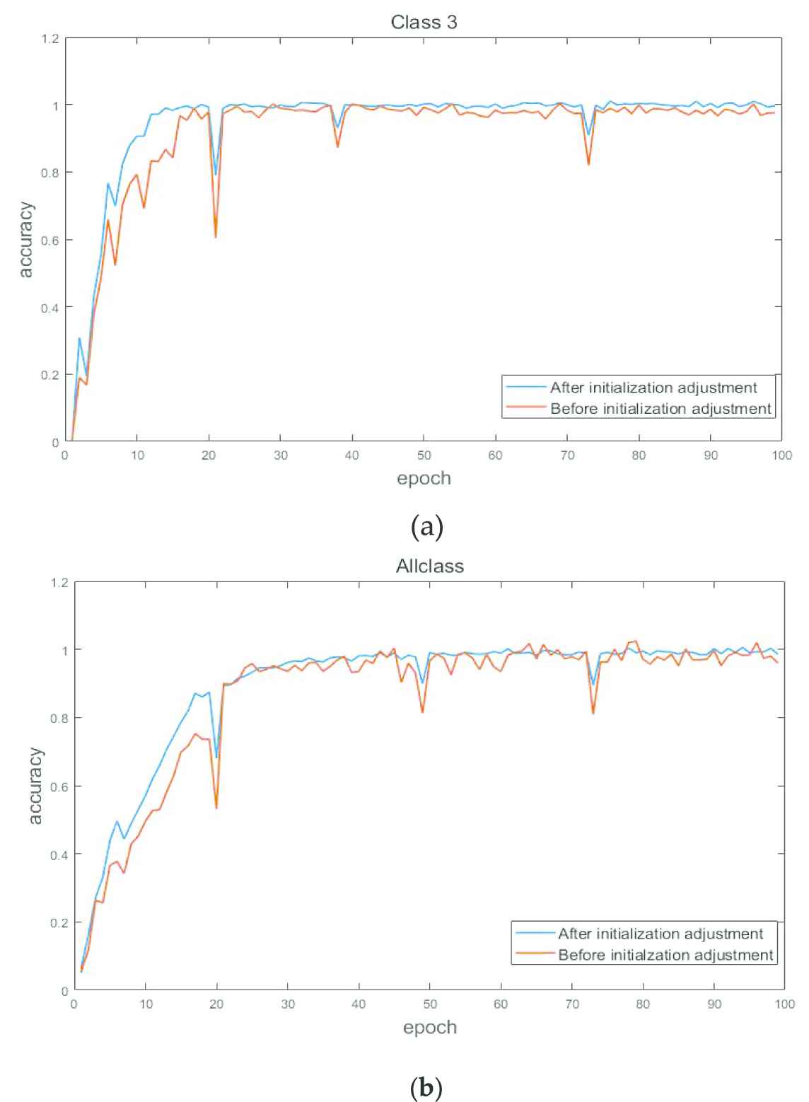
Training process under different initialization of RBM weights. (a) Class 3 and (b) All class.
5.4.3. Key parameters of KPCA-DBN
Parameters selection is very important in training model of KPCA-DBN and some of them are determined based on above analysis. We choose linear kernel function, 100 principal components, a three-layer structure and 100 nodes of hidden layer. The number of nodes in hidden layer is equal to that of input layer nodes. The results of fault diagnosis normally can be further improved by setting preferred parameters value in training DBN. The training process is affected easily by parameters of loss detection period and iterations from our experience. Loss detection period (number of batch training) is defined as 5, 10, 20 or 30 for comparisons and the maximum iterations are chosen to be 1000, 2000, 3000, 4000, 5000 or 10000. The experimental data are from “All class” and each experiment is repeated 5 times. In Figure 11, x axis is divided into four segments to show the results of different loss detection periods and the results obtained by KPCA-DBN in different maximum iterations are marked by six colors. The training time is plotted as bar graph and diagnosis accuracy is plotted as line graph.
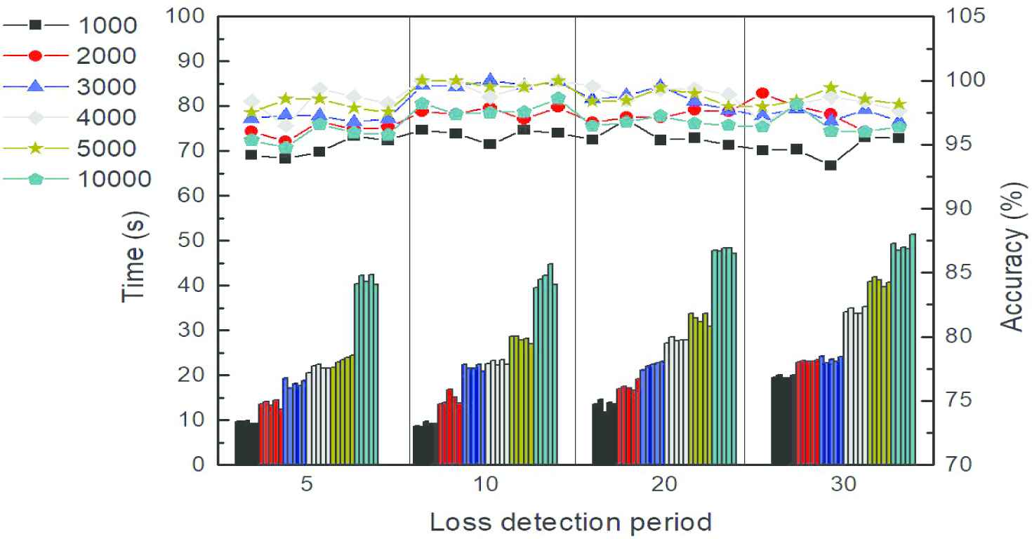
Diagnosis results of training process with different loss detection period and maximum iteration.
Compared heights of same color bars in Figure 11, training time is 9.42s, 13.72s, 18.03s, 20.92s, 22.80s or 41.41s in different iterations when loss detection period is 5. When loss detection period is 30, training time is 19.87s, 21.03s, 23.73s, 33.85s, 41.26s or 49.41s. We can conclude that training time increase with increase of loss detection period. For diagnosis accuracy, values of points in the six lines in the first segment of x axis are smaller than those in other segments. As loss detection period increases to 10, the value of each point in the blue line is almost equal to 99%. Nevertheless, when loss detection period is increase to 30 the lowest testing accuracy is only 93.3% (336/360) and six lines fluctuate greatly, which indicates accuracy falls and stability of calculation decreases. Loss detection period represents how many training times are taken before checking error to confirm whether to stop training. If loss detection period is too large, weights of RBM cannot be updated frequently enough, which leads to inadequate learning and more calculating time. Conversely, it is easy to fall into local optimum and reduce the generalization.
From Figure 11, black line is almost at the bottom of six lines. In the line, the maximum value is 96.9% (349/360) and the minimum one is 93.3% (336/360), which shows wider wave range than other lines. We can conclude that when the number of iterations is 1000, the performance of classifier is sensitive to loss detection period. Therefore, classifier remains undertrained in 1000 iterations so that the performance of classifier is poor and easily affected by parameters in training process. When number of iterations is 3000, the classifier has been almost adequately trained and the average accuracy can reach 98.4%. The average accuracy is close to 99.1% and testing results are stable until it increases to 5000. While iteration is increased to 10000, testing accuracy is not improved instead of degradation of stability. The testing accuracies are 96.4% (347/360), 98% (347/360), 96.1% (346/360), 95.8% (345/360), 96.4% (347/360) in 10000 iterations as loss detection period is 30. We can conclude that fitting error is small enough when the number of iterations is 5000. If continue to increase iterations, there is little improvement on classification accuracy and even decline in efficiency and classifier stability.
Loss detection period and iterations are two key parameters for training DBN and they are set depended on complexity and sizes of samples. In this paper, when the loss detection period is 10 and the number of iterations is 3000, DBN can be fully trained to achieve high efficiency and high accuracy of both training and testing.
6. CONCLUSIONS
An approach of KPCA- DBN is proposed to solve the problem of low recognition rate and long training time for detecting incipient faults submerged in strongly noisy background.
The method of VMD-Sample entropy–wavelet threshold denoising is effective to separate noises from raw data and SNR of vibration signals of rolling bearing is obvious improved. The denoised signals are transformed by Hilbert transform and FFT to form the frequency-domain experimental signals. A KPCA-DBN method is used to diagnose incipient faults of rolling bearings.
Firstly, kernel function is introduced to perform nonlinear operation in mapping space and principal components of experimental signals are preserved. Secondly, principal components are made input signals of DBN to diagnose sizes and locations of incipient faults of rolling bearings. The improved DBN through network simplification and weight initialization adjustment is used as feature extractors to learn and extract representative features of training data. During unsupervised self-learning process, weights of DBN are adjusted in reverse by BP and Softmax is constructed in the last layer to output classification results. The results are shown as follows:
The proposed method of KPCA-DBN can automatically retain the principal components that represent data characteristics according to data distribution without depending on manual feature extraction by expert experience. The method reduces data dimension and eliminates interference information.
The model of combining of KPCA and DBN can shorten network structure and increase convergence rate. Identification accuracy achieved by KPCA-DBN with only two hidden layers and fewer nodes comes up to that by DBN with three hidden layers and more nodes. Weights of DBN are initialized by contribution rate of principal components calculated by KPCA, which accelerates the convergence rate of the network.
By optimizing parameters of KPCA-DBN, the average test accuracy by KPCA-DBN reaches 99.1% for identification of 12 labels including incipient faults and the training time is 28s which is half of that by DBN model. The locations detection of incipient faults on outer race gets to average accuracy of 98.9%. Besides, the average accuracy of fault size detection is above 99%.
The calculation results show the proposed method is superior to other existing intelligence diagnosis methods including BP, SVM, KNN, Deep-EMD-PCA, CNN-SVM and traditional DBN in meeting real-time fault diagnosis.
The paper provides an application in detecting sizes and locations of incipient faults of rolling bearings by the proposed method. However, it is also especially suitable for rotating equipment with high requirement for operation safety, such as rolling bearing of axle box in high-speed emu or main shaft bearing of aircraft engines. These rotating equipment are required to have efficient judgment on incipient faults during operation, which provides effective guarantee to avoid malignant development of the faults. The proposed method is also universal for multi-task classification and it can be applied to other scenarios as well because of the ability of automatically learning.
CONFLICTS OF INTEREST
The authors declare they have no conflicts of interest.
AUTHORS' CONTRIBUTIONS
The study is guided by Haifeng Huang and written by all authors.
Funding Statements
This work was supported by the Sichuan Science and Technology Program (grant number 19GJHZ0061).
REFERENCES
Cite this article
TY  - JOUR
AU  - Heli Wang
AU  - Haifeng Huang
AU  - Sibo Yu
AU  - Weijie Gu
PY  - 2021
DA  - 2021/05/28
TI  - Size and Location Diagnosis of Rolling Bearing Faults: An Approach of Kernel Principal Component Analysis and Deep Belief Network
JO  - International Journal of Computational Intelligence Systems
SP  - 1672
EP  - 1686
VL  - 14
IS  - 1
SN  - 1875-6883
UR  - https://doi.org/10.2991/ijcis.d.210518.002
DO  - 10.2991/ijcis.d.210518.002
ID  - Wang2021
ER  -