
The Value Function with Regret Minimization Algorithm for Solving the Nash Equilibrium of Multi-Agent Stochastic Game
 , Wensheng Jia*
- DOI
- 10.2991/ijcis.d.210520.001How to use a DOI?
- Keywords
- Regret minimization; Multi-agent; Stochastic game; Nash equilibrium; Spatial prisoner's dilemma
- Abstract
In this paper, we study the value function with regret minimization algorithm for solving the Nash equilibrium of multi-agent stochastic game (MASG). To begin with, the idea of regret minimization is introduced to the value function, and the value function with regret minimization algorithm is designed. Furthermore, we analyze the effect of discount factor to the expected payoff. Finally, the single-agent stochastic game and spatial prisoner's dilemma (SDP) are investigated in order to support the theoretical results. The simulation results show that when the temptation parameter is small, the cooperation strategy is dominant; when the temptation parameter is large, the defection strategy is dominant. Therefore, we improve the level of cooperation between agents by setting appropriate temptation parameters.
- Copyright
- © 2021 The Authors. Published by Atlantis Press B.V.
- Open Access
- This is an open access article distributed under the CC BY-NC 4.0 license (http://creativecommons.org/licenses/by-nc/4.0/).
1. INTRODUCTION
Fudenberg and Levine [1] put forward the game learning theory, the goals of the bounded rationality agents are to maximum their long-term payoff and regret minimization by constantly adjusting their strategies from their known information. Recently, many scholars focused on the study Nash equilibrium (NE) of multi-agent stochastic game (MASG). Yang and Wang [2] researched the multi-agent reinforcement learning (MARL) from the perspective of game theory. Rubinstein [3] investigated that bounded rational participants continuously modified their cognition in repeated games in which compared current strategies with previous ones to make optimal strategy choices. Asienkiewicz and Balbus [4] presented the existence analysis of NE for random games under certain conditions. Watkins [5,6] first proposed the Q-learning method, and proved the convergence of Q-learning. Littman [7] proposed a minimax Q-learning for two-person zero-sum stochastic game. Shoham et al. [8] discussed Nash-Q learning in general-sum stochastic game. Therefore, Q-learning and various improved learning algorithms play an important role in the implementation of NE for the MASG.
Reinforcement learning [9] solved the MASG by interacting with complex environment and learning from experiences. Bowling and Velson [10,11] proposed a classic method to evaluate MARL algorithm. The MARL has recently been extensively used in wireless sensor networks [12], event-triggered consensus system [13], traffic signal controllers [14], numerical algorithm [15], comparative analysis [16], integrodifferential algebraic [17], computational algorithm [18], and other fields. But the majority MARL algorithms either lack a rigorous convergence guarantee [19], potentially converge only under strong assumptions such as the existence of an unique NE [20,21], or provably non-convergent in all cases [22]. Zinkevich [23] identified the nonconvergent behavior of the value-function method in general-sum stochastic game. Minagawa [24] considered a sufficient condition for the uniqueness of NE in strategic-form game. However, Hansen et al. [25] proposed the concept of no regret to measure convergence, which came up with a new criteria to evaluate convergence in zero-sum self-plays [26,27]. Regret minimization has been used in a variety of games in recent years [28]. Inspired by research works mentioned above, we mainly studies the value function with regret minimization algorithm for solving the NE of MASG. The central idea of regret minimization is that the agent obtained a payoff after the agent has taken an action in the learning process, agents can retrospect the history of actions and payoff taken so far, and the agent regret not having taken another action, namely, the best action in hindsight. The agents' goal is to minimize the cumulative regret, written as the sum
The remainder of this paper is structured as follows: in Section 2, we introduce the model of MASG, and analyze the discount factor to the influence of discounted expected payoff. In Section 3, the idea of regret minimization is introduced to the value function, and the value function with regret minimization algorithm is designed. In Section 4, a simple stochastic game and the SDP game are investigated in order to support the theoretical results. Finally, we present some brief summaries.
2. PROBLEM DESCRIPTION AND PREREQUISITES
2.1. The Model of Multi-Agent Stochastic Game
A framework of MASG is given as follows [7]:
Let
In infinite-horizon process [9], the agents' discounted payoff from time step t to horizon is,
The model of MASG as shown in Figure 1.
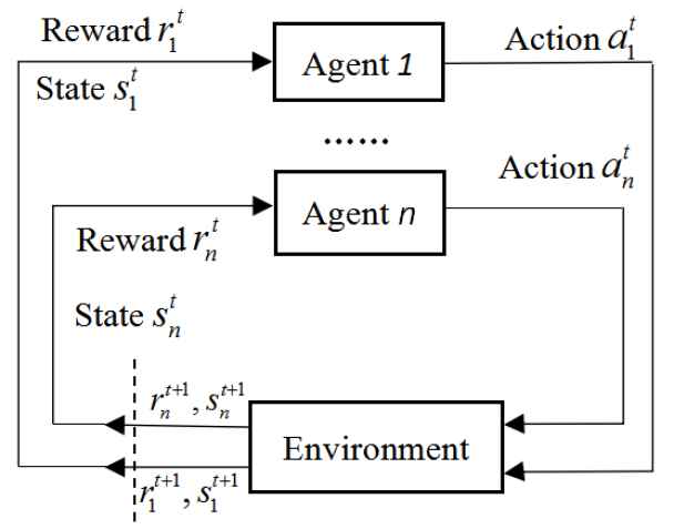
The interaction of multi-agent and environment.
The optimal value function of agent i is defined by
Definition 2.1.
(Nash equilibrium NE of the MASG) Let
2.2. The Analysis of Discount Factor
For a Markov decision process (MDP) system, we consider the discount factor to the influence of the expected payoff in MASG. Now we make a simple experiment about the MASG
Meanwhile,
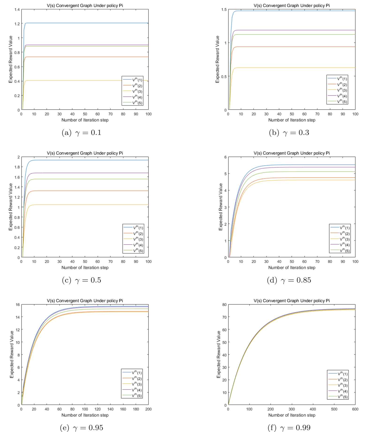
The diagram of the convergence of the value function under different discount factor.
According to Figure 2(a–f), we can observe that starting from
3. THE VALUE FUNCTION WITH REGRET MINIMIZATION ALGORITHM
3.1. The Cumulative Regret Minimization
Assuming that the finite-horizon, a policy
where
In Bubeck [30], the formula (6) is the normalized object. The loss
We define the cumulative regret minimization of all agents in the MASG as follows:
3.2. Arithmetic Flow of the Value Function with Regret Minimization Algorithm
The implementation steps of the value function with regret minimization algorithm are as follows:
step 1: Initialization parameters. Some strategies are randomly generated, and set the discounted factor, the value of cumulative regret degree is
step 2: Each agent's the value function
step 3: The cumulative regret degree
step 4: Stopping condition of iterations: does the cumulative regret degree satisfy
Once the optimal strategy is obtained by satisfying the cumulative regret, the value of the discounted expected payoff is defined. The value function under the regret minimization algorithm see Figure 3.
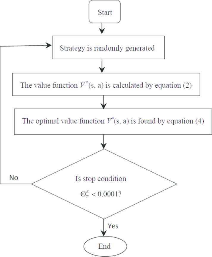
Flow chart of value function under regret minimization algorithm.
4. THE NEOF A MASG
4.1. A Simple Stochastic Game
The aim of the agent is to maximize their long term discounted expected payoff making respond to others agents. We give an example of a SASG as follows:
Example 1.
Let
The above description can be shown in Table 1. We suppose that the horizon is T and the final payoff is
| Agent(N) | 1 | |||||
|---|---|---|---|---|---|---|
| State( |
||||||
| Action( |
– | |||||
| Payoff( |
2 | 3 | 5 | 10 | – | 0 |
| Transition probability( |
(0.0, 1.0, 0.0) | (1.0, 0.0, 0.0) | (1.0, 0.0, 0.0) | (0.0, 0.5, 0.5) | – | (0.0, 0.0, 1.0) |
The SASG was described in Example 1.
Assume that the decision will be made at
By the backward induction method, at time
So
So
At time
So
So
At time
So
So
Therefore, the optimal value function and the optimal strategy in any state as follows,
4.2. The Spatial Prisoners' Dilemma
The SPD [32] can be regarded as a two-agent two-action stochastic game
Example 2.
Let
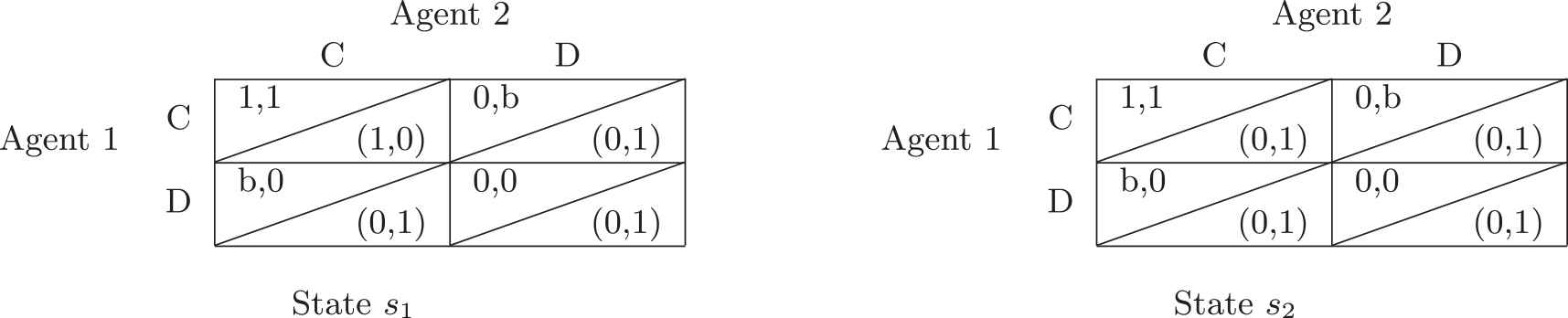 |
The description of the MASG, where state
The game starts in state
In state
| Agent 1 | |||
| C |
D |
||
| Agent 2 | C | 1 + |
|
| D | b + |
||
or
| Agent 1 | |||
| C |
D |
||
| Agent 2 | C | 1 + |
|
| D | b + |
||
where
Evidently,
Assume that both of agents select Cooperation in state
Meanwhile,
On the one hand,
Therefore, we simulate the SDP on a 300
From Figure 4(a–f) we can see the number of cooperators suddenly dropped owing to agents being isolated and surrounded by defectors, hence a few cooperators that survive will create small clusters and then rise in numbers, so the cooperators quickly become dominant over the defectors after a few generations when the temptation factor
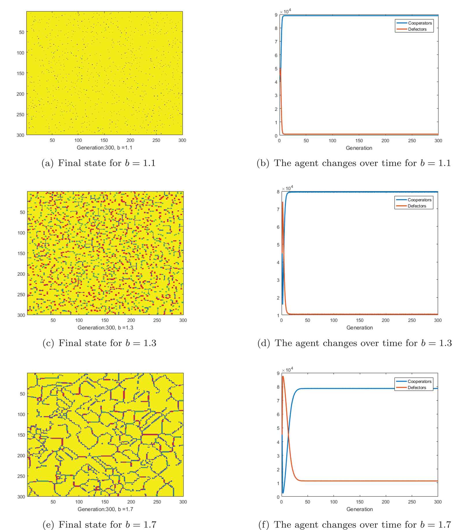
The agent strategy change with different
Up until
According to Figure 5(a–d), when
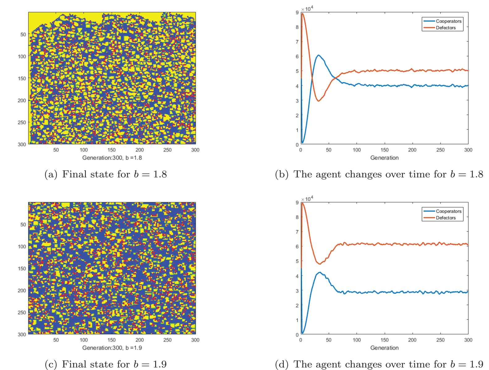
The agent strategy change with different
5. CONCLUSION
In this paper, we give a new attempt to solve NE of MASG by using the value function with regret minimization algorithm. We consider the expected payoff as an optimization criterion between agents. To begin with, the idea of regret minimization is introduced to the value function, and the value function with regret minimization algorithm is designed. Furthermore, we analyze the effect of discount factor to the discounted expected payoff. Finally, the simulation results show that when the temptation parameter is small, the cooperation strategy is dominant; when the temptation parameter is large, the defection strategy is dominant, we improve the level of cooperation between agents by setting appropriate temptation parameters
CONFLICTS OF INTEREST
The authors declare they have no conflicts of interest.
AUTHORS' CONTRIBUTIONS
All authors read and approved the final manuscript
ACKNOWLEDGMENTS
This work was supported by the National Natural Science Foundation of China (Grant No. [12061020], [71961003]), the Science and Technology Foundation of Guizhou Province (Grant No.20201Y284, 20205016, 2021088), the Foundation of Guizhou University (Grant No. [201405], [201811]). The authors acknowledge these supports.
REFERENCES
Cite this article
TY  - JOUR
AU  - Luping Liu
AU  - Wensheng Jia
PY  - 2021
DA  - 2021/05/26
TI  - The Value Function with Regret Minimization Algorithm for Solving the Nash Equilibrium of Multi-Agent Stochastic Game
JO  - International Journal of Computational Intelligence Systems
SP  - 1633
EP  - 1641
VL  - 14
IS  - 1
SN  - 1875-6883
UR  - https://doi.org/10.2991/ijcis.d.210520.001
DO  - 10.2991/ijcis.d.210520.001
ID  - Liu2021
ER  -