
A Comprehensive Study of Machine Learning Methods on Diabetic Retinopathy Classification
 , Omer Faruk Beyca1, , Onur Dogan2, 3,
 - DOI
- 10.2991/ijcis.d.210316.001How to use a DOI?
- Keywords
- machine learning; ensemble learning; transfer learning; XGBoost; PCA; SVD
- Abstract
Diabetes is one of the emerging threats to public health all over the world. According to projections by the World Health Organization, diabetes will be the seventh foremost cause of death in 2030 (WHO, Diabetes, 2020. https://www.afro.who.int/health-topics/diabetes). Diabetic retinopathy (DR) results from long-lasting diabetes and is the fifth leading cause of visual impairment, worldwide. Early diagnosis and treatment processes are critical to overcoming this disease. The diagnostic procedure is challenging, especially in low-resource settings, or time-consuming, depending on the ophthalmologist's experience. Recently, automated systems now address DR classification tasks. This study proposes an automated DR classification system based on preprocessing, feature extraction, and classification steps using deep convolutional neural network (CNN) and machine learning methods. Features are extracted from a pretrained model by the transfer learning approach. DR images are classified by several machine learning methods. XGBoost outperforms other methods. Dimensionality reduction algorithms are applied to obtain a lower-dimensional representation of extracted features. The proposed model is trained and evaluated on a publicly available dataset. Grid search and calibration are used in the analysis. This study provides researchers with performance comparisons of different machine learning methods. The proposed model offers a robust solution for detecting DR with a small number of images. We used a transfer learning approach, which differs from other studies in the literature, during the feature extraction. It provides a data-driven, cost-effective solution, which includes comprehensive preprocessing and fine-tuning processes.
- Copyright
- © 2021 The Authors. Published by Atlantis Press B.V.
- Open Access
- This is an open access article distributed under the CC BY-NC 4.0 license (http://creativecommons.org/licenses/by-nc/4.0/).
1. INTRODUCTION
Diabetic retinopathy (DR) is one of the most common retinal diseases and is a leading cause of blindness among people aged 20 to 65, worldwide. The risk of blindness in DR patients is 25 times higher than that of healthy people [1]. DR is the most common microvascular complication in diabetes. The reported prevalence of DR in people with diabetes is around 40%. It is more common in Type-1 diabetes than in Type-2. DR is mainly microangiopathy, in which small blood vessels are particularly vulnerable to damage from high glucose levels. DR is a progressive process and has several degrees: background DR, diabetic maculopathy, pre-proliferative DR, proliferative DR, and advanced diabetic eye disease. This categorization is widely used in clinical practice. There are several indications of DR, including microaneurysms, retinal haemorrhages, exudates, diabetic macular oedema, cotton wool spots, venous or arterial changes, ischemic maculopathy. The duration of diabetes, poor control, pregnancy, hypertension, obesity, smoking, cataract surgery, and anemia are some of the risk factors [2].
Parallel to an increase in the spread of diabetes, the number of DR patients has also increased. In the current clinical diagnosis, ophthalmologists examine retinal images of patients and evaluate the condition. It is a time-consuming process. Additionally, there is a lack of medical resources (such as equipment and specialists) in some countries and so DR cannot be diagnosed and treated in a timely manner. Even if there were enough ophthalmologists in a city, misdiagnosis often occurs because of a lack of experience. On the other hand, developments in imaging technologies enable more medical data production. Automatic screening and grading of DR is necessary to overcome these problems and process large amounts of data quickly and accurately.
Recently, automated systems (which are generally based on artificial intelligence), have made remarkable achievements in many areas. One of these areas is medicine. Deep neural networks, particularly convolutional neural networks (CNNs), have outstanding performance in computer vision tasks that learn representative and hierarchical image features from a sufficient number of images. CNNs have the capability to process and analyze fundus images automatically and accurately [3–5].
Training deep learning models from scratch requires sufficient resources, such as high processing or memory capacity, to process large amounts of data; this can be costly to collect and label. Medical data is one of the most prominent types of such data. These problems can be addressed by transfer learning, which is a frequently used technique in deep learning. The basic idea of transfer learning is that a model is developed for a task and is then re-used as a starting point for another task model. Learning knowledge is transferred between tasks. Depending on the relevance of the tasks, there are various uses for transfer learning. For example, a pretrained network can be used in feature extraction from new samples, or to fine-tune them.
Transfer learning is applied to many computer vision tasks. DR classification with limited amounts of data is one of these tasks. There are many well-performing models trained on ImageNet data, which presents a standard computer vision benchmark dataset. VGG19, ResNet50, InceptionV3, MobilNet, and DenseNet121 are some of these models. InceptionV3 is one of the most used models in DR classification studies. The high performance of InceptionV3 may be associated with the inception module, which was found to be very useful in DR images [6].
This study proposes an automated DR classification system based on the preprocessing of images, feature extraction, and classification steps. Features are extracted from the InceptionV3 model using the transfer learning approach and this differs from other studies in the literature. The extracted features are classified by several machine learning methods, namely XGBoost, Bagged Decision Trees, Random Forest, Extra Trees, Support Vector Machines, Logistic Regression, and multilayer perceptron. We show that, when extracting generic descriptors from one of the initial layers of InceptionV3, competitive classification accuracy can be acquired with machine learning methods without layer-wise tuning. Moreover, our approach offers satisfactory results when considering the number of pre-processing methods used, the model's complexity, the number of parameters to be trained, and the computation and memory capacity needed. This study provides researchers with a performance comparison of different machine learning methods.
The rest of the paper is organized as follows. Section 2 outlines the related work in the literature. Section 3 outlines the materials and methods used in this study. Experimental results and discussions are given in Section 4. Lastly, the conclusions are presented in Section 5.
2. RELATED WORK
In the literature, some studies classify DR by detecting lesions such as exudates, hemorrhages, microaneurysms, etc., or by segmenting blood vessels with various techniques. During the identification and segmentation of DR signs or calculating some numerical indexes from DR images, manual, and automatic feature extraction methods are applied. Many studies apply manual methods (in which variables are measured manually), or hand engineering features are extracted using various image processing techniques or separate algorithms, such as HOG and SIFT. Manual efforts bring extra complexity and instability [7–10].
Early studies on DR classification are mainly based on extracting features of retinal images with hand engineering methods and classifying them with machine learning methods. Kasurde and Randive [11] proposed a proliferative DR detection model. This type of DR can be detected by tracking the growth of abnormal vessels. The proposed model is based on vessel segmentation, straight vessel detection using morphological operations and structuring elements, removing straight vessels, and then obtaining abnormal vessels. Lastly, the images are classified according to vessel pixel statistics.
Dhanasesekaran et al. [12] preprocessed retinal images and then segmented them using the Fuzzy C-means segmentation technique. The authors extracted features using the Gabor Filter and Gaussian Mixture Model and then used them in classification. Omar et al. [13] classified DR images by detecting DR features, namely hemorrhages, exudates, and blood vessels. The process stages were pre-processing, vessel and hemorrhage detection, optic disc removal, and exudate detection. The authors used morphological operations in detection. Classification is made by taking into consideration the lesion locations or some statistical measures. Similarly, Punithavathi and Kumar [14] used morphological operations to extract the number of microaneurysms and texture features. These features are then classified by the Extreme Learning Machine classifier.
Sayed et al. [15] classified DR images with support vector machines and probabilistic neural network algorithms. The authors extracted features using grayscale conversion, discrete wavelet transform, adaptive histogram equalization, matched filter, and fuzzy C-means segmentation. Sisodia et al. [16] preprocessed retinal images by applying green channel extraction, histogram equalization, image enhancement, and resizing techniques. The authors obtained fourteen features for quantitative analysis. Classification was performed by examining the mean value and standard deviation of extracted features. Sreng et al. [17] segmented possible lesions of DR using a combination of pre- and postprocessing steps. The authors obtained eight feature sets, such as morphological features, color features, pattern features, and first-order statistical features. The optimal feature set was selected by applying the hybrid simulated annealing method. An ensemble bagging classifier was used in the binary classification task. Reddy et al. [18] applied an ensemble-based machine learning model including logistic regression, decision tree, random forest, adaboost, and k-nearest neighbor Classifiers on the DR dataset from the UCI machine learning repository. The model was trained on normalized datasets and the proposed ensemble-based model performed better than the individual machine learning algorithms.
Recently, deep learning methods have become popular in DR classification studies. These methods can learn features directly from images. Vo and Verma [19] proposed two deep, CNNs, namely VGGNet with extra kernel (VNXK) and combined kernels with multiple losses network (CKML Net). The authors also introduced a hybrid colour space. They conducted a referable/non-referable classification of DR on the Messidor dataset. Transfer learning was used to handle the imbalanced dataset and experiments of the proposed nets were carried out on the hybrid color space. Li et al. [3] extracted features from various pretrained deep learning models and used a support vector machine to classify images in Messi-dor data. Sahlsten et al. [4] proposed a deep network based on the InceptionV3 model to distinguish DR and macular edema features. The authors made a binary classification of DR [referable diabetic retinopathy (RDR) vs. non-referable diabetic retinopathy (NRDR)]. Experiments were undertaken by varying input image sizes using the Messidor dataset. The authors compared the results of an ensemble-based model and a single model.
Kassani et al. [20] proposed a method that is based on an aggregation of multilevel features from different convolution layers of Xception. Extracted features were fed into a multilayer perceptron to classify DR images. Additionally, transfer learning strategy and hyperparameter tuning were used to improve classification performance. The Kaggle APTOS 2019 contest dataset was used in the experiments. Mateen et al. [21] proposed a DR classification system using a Gaussian mixture model for region segmentation, VGGNet for feature extraction, singular value decomposition (SVD) and principal component analysis for feature selection. Softmax was used for fundus image classification. Bodapati et al. [22] extracted features of DR images from multiple pre-trained ConvNet models, such as VGG16, Xception. The authors blended these features to get the final feature representations, which are used to train a deep neural network. Experiments were carried out on the Kaggle APTOS 2019 contest dataset. Doshi et al. [23] used various downscaling algorithms before feeding the retinal images into a Deep Learning Network for classification. The authors proposed a Multi-Channel InceptionV3 model and used EyePACS and Indian Diabetic Retinopathy Image Datasets in experiments.
Gargeya and Leng [24] proposed a custom CNN model for DR diagnosis. Features were extracted from the global average pooling (GAP) layer of the proposed network. Some metadata information is added to the extracted features to increase the accuracy of prediction. A gradient boosting classifier was applied for diagnosis and the model trained with the EyePACS dataset. The proposed model achieved an AUC (Area Under Curve) of 94% for no-DR vs. any DR grade and AUC of 83% for no-DR vs. mild DR on Messidor-2. Voets et al. [25] trained an InceptionV3 model for detecting RDR. The images were preprocessed, and data augmentation was used. The authors used ensemble learning by training ten networks and the final prediction was then made by calculating the mean of the predictions. The EyePACS dataset, hosted on the Kaggle platform, is used in training and testing. The algorithm gives an AUC of 85.3% on Messidor-2.
de La Torre et al. [26] suggested a CNN model comprising 17 layers. The authors used the EyePACS dataset hosted on the Kaggle platform to train the model. Some data augmentation techniques were applied to artificially equalize the training set. The binary classification accuracy of the model for predicting the most severe DR (grouping classes 2, 3 and macular edema) is 91.0% on Messidor-2.
Toledo-Cortés et al. [27] suggested a deep learning gaussian process (GP) for DR classification. The pretrained InceptionV3 model was used as a feature extractor and fine-tuned with the EyePACS dataset. A GP regressor was applied in diagnosing the RDR images and the model gave an AUC of 87.87% on Messidor-2.
Saxena et al. [28] experimented with different Inception and ResNeT-based models. Inception Res-NetV2 outperformed all of the other versions of the models. The authors trained multiple models on a different train and validation sets from the Eye-PACS dataset by arbitrary splitting. The results of these models were combined using ensemble averaging methods and Messidor-2 was used as a benchmark test dataset. A binary classification was made: no-DR vs. any DR grade. The model gives an AUC of 92% on Messidor-2 with a specificity and sensitivity of 86.09% and 81.02%, respectively.
Zago et al. [29] suggested a patch-based CNN model to classify DR images. The model learns to detect lesions (localization) on a given image. A selection model, which is a five-layer CNN model, selects the patches. The authors used VGG16, which was initialized with pre-trained weights and tuned using the selected patches. The DIARETDB1 dataset was used in training. The model was trained with 51,840 lesion and nonlesion patches and gave an AUC of 94.4% on Messidor-2, for detecting RDR.
Tseng et al. [30] developed fusion CNN architectures. The best performing architecture trained an object detection model based on RetinaNet. An object detection model was used to enhance the major symptoms of potential DR regions. InceptionV4 and DenseNet121 were used in feature extraction. The extracted features were then concatenated and ridge regression applied to classify the images. The authors used a private dataset from Taiwanese Hospitals and used Messidor-2 for benchmarking. The model achieved an accuracy of 91.99% in detecting RDR on Messidor-2.
The performance comparison of studies on Messidor-2 in the detection of various degrees of DR is given in Table 1. According to Table 1, the proposed model with an AUC of 93.55% and accuracy of 91.40% has comparable results to previous studies in a binary classification task. These previous studies used other publicly available, or custom datasets, with significantly more observations in the training phase and used Messidor-2 as a benchmark dataset. In the proposed model, we used Messidor-2, a very small dataset, in training and testing. The proposed model gives a robust performance with a small dataset, which constitutes good value, considering the difficulties in collecting large quantities of labeled images, the training time, and computational power required.
| Study | Model | Training Data (Number of Images) | Classes | Performance (%) |
|---|---|---|---|---|
| Gargeya and Leng [24] | CNN + Gradient Boosting | EyePACS (75137) | No-DR vs. DR | 94.0 (AUC) |
| Voets et al. [25] | InceptionV3 CNN | EyePACS in Kaggle (45717) | NRDR vs. RDR | 85.3 (AUC) |
| de La Torre et al. [26] | CNN | EyePACS in Kaggle (75650) | Most severe cases of DR vs. the rest | 91.0 Acc. |
| Toledo-Cortés et al. [27] | InceptionV3 + GP regressor | EyePACS (56827) | NRDR vs. RDR | 87.87 (AUC) |
| Saxena et al. [28] | Inception and ResNeT based models | EyePACS (56839) | No-DR vs. DR | 92.0 (AUC) |
| Zago et al. [29] | Patch-based CNN | DIARETDB1 (28) | NRDR vs. RDR | 94.4 (AUC) |
| Tseng et al. [30] | Fusion CNN Architecture | Custom (22617) | NRDR vs. RDR | 91.99 Acc. |
| Proposed Model | InceptionV3 + XGBoost | Messidor-2 (1392) | NRDR vs. RDR | 91.40 Acc.; 93.55 (AUC) |
Performance comparison on Messidor-2 in detection various degrees of DR.
3. METHODOLOGY
3.1. Convolutional Neural Networks
CNNs are specialized types of neural networks and can be applied to many kinds of data with different dimensions. CNN includes three kinds of layers: convolutional, pooling, and fully connected layers. Convolutional layers constitute the main building blocks of a CNN and summarize the features in an image [31].
The network uses a mathematical operation, which is called convolution. Convolution is a kind of linear operation which includes multiplying a set of weights with input data. Convolutional layers are composed of filters and feature maps. Filters are basically the neurons of the layer and act like a neuron; filters have weighted inputs and produce an output value. A feature map is generated from the output of one filter applied to the previous layer. A given filter is slid over the entire previous layer. Each position results in the activation of the neuron and the outputs form the feature map. Pooling layers can be considered to be a technique that compresses or generalizes feature representations. They downsample feature maps. The result of applying a pooling layer gives a summarized version of the features. Lastly, fully connected layers are classic feedforward neural network layers [32].
CNNs are sensitive to the spatial coherence or local pixel correlations in images. So they are preferred in many image classification, recognition or analysis problems. Recently, CNNs have offered valuable insights into various medical applications but there are some challenges when using CNNs in medical tasks [1]. It is difficult to collect medical images of good quality and sufficient numbers. The availability of labeled data is limited. Collecting and labeling data is a time-consuming process; besides, correct labeling is critical and depends on specialist experience [3,5,33,34]. Signs of DR (such as microaneurysms, retinal hemorrhages, and exudates) are complicated in a fundus image. There are common signs that are shared with the other retinal vascular diseases. Some small signs are difficult to see if image quality is poor. High classification accuracy is difficult to attain by a single model with a small number of datasets. Two essential strategies are used in deep learning studies to overcome the mentioned challenges: transfer learning and ensemble learning [1].
3.2. Transfer Learning
A common approach in deep learning for a small number of image datasets is using a pretrained network, which is a saved network. Transfer learning transfers knowledge learned in a pretrained network to increase the learning performance of a target task. Transfer learning is generally referred to when there is not enough dataset for the target domain training process or when there is a favorable solution to a related problem. It would be advantageous to use such knowledge to solve the target problem [35]. Transfer learning is used to train a CNN by not initializing CNN weights from scratch. Instead, weights are imported from another CNN, which is trained on a large dataset. The ImageNet dataset is the most famous dataset for transferring weights of trained models [6].
Pretrained networks are composed of two parts. The first part includes a series of convolution and pooling layers and these layers end with a densely connected classifier. Convolutional feature maps take into consideration object locations in an input image. On the other hand, densely connected layers at the top of the convolutional base are mostly useless for object detection problems. A pretrained network is trained on a large dataset, generally on large-scale image classification problems. These kinds of networks include VGG19, Xception, MobilNet, ResNet, DenseNet, and InceptionV3. These networks were trained on the ImageNet dataset, in which classes are mostly everyday objects and animals. If the dataset is large and general enough, pretrained networks can be used as generic models by learning the spatial hierarchy of features. Thus, these networks can be useful for many different computer vision tasks, even if new tasks consist of entirely different classes [35].
There are two ways to use a pretrained model: feature extraction and fine-tuning. Feature extraction is based on using the convolutional base of a pretrained network with a new classifier and running the new dataset through it. The convolutional base is reusable because it learns representations that are generic for various tasks. Complementary to feature extraction, is fine-tuning, where some of the top layers of the frozen model base (used for feature extraction) are unfrozen. The top layers and classifier parts of the model are then jointly trained [35,36].
Transfer learning from a pretrained CNN model is shown in Figure 1. The trained convolutional base can be used as a feature extractor and then extracted features are fed into a new classifier. On the other hand, depending on the relevance of the tasks, layer-wise fine tuning can be carried out on the convolutional base by unfreezing some of the layers.
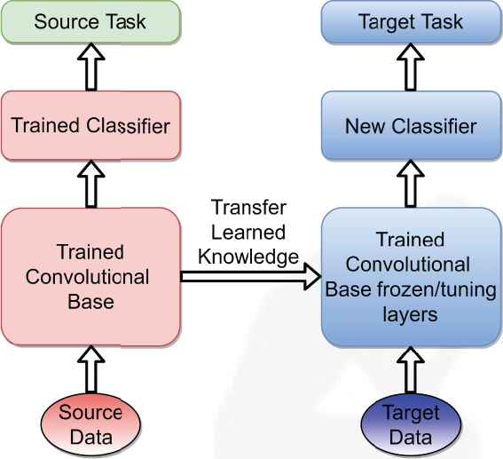
Transfer learning from a pretrained convolutional neural network (CNN) model.
Using full scale, fine-tuned transfer learning methods has two main issues: negative transfer and overfitting. When the domain of the pretrained network and the target outputs are not similar we may see a performance decrease in the transfer learning model, which is called negative transfer [37]. This is because features extracted in the later layers are complex and not suitable for the target domain. On the other hand, fine-tuning later layers can lead to overfitting problems. In order to adapt later layer features to our target domain we need to train the layers with a huge number of parameters. This is not practical since the common, pretrained network InceptionV3 has 21,802,784 parameters; ResNet152 has 58,370,944 parameters. When these large-scale networks are trained, there is the risk of overfitting the model; it is also extremely time and CPU power consuming. In order to tackle these problems, we only use features from earlier layers. Early features are primitive and do not depend on the domain which can be used in machine learning algorithms as inputs [35,38].
The suitability of transfer learning for DR classification can be evaluated by comparing a model that was trained from scratch, to its fine-tuned version. Several studies (such as Masood et al. [39]; Wan et al. [5]; Xu et al. [40]) agree that using transfer learning increases the accuracy of a model significantly in the classification of DR [6]. A vast number of images are needed to sufficiently train a deep learning model. DR image datasets have a limited number of images. Collecting DR images and labelling them correctly is a very costly process in terms of time, experience, and resources. We used transfer learning in the proposed study because of the dataset limitation and its proven success in DR classification.
InceptionV3 is a frequently-referenced, deep CNN model, and is a feature extractor in DR classification studies. The superior performance of InceptionV3 refers to some network connection techniques, such as using MLPconv layers to replace linear convolutional layers, adopting batch normalization, and factorizing convolutions with large kennel sizes. These techniques significantly decrease the number of parameters and the complexity of the model [10]. In this study, we also used InceptionV3 as a feature extractor to generate feature vector representations from retinal images.
3.3. Ensemble Learning
Ensemble learning methods try to improve generalizability or robustness over a single estimator by combining the multiple model predictions. Bagging, boosting, and stacking models are based on ensemble learning. When the training dataset is small, ensemble methods can decrease the risk of choosing a weak classifier by averaging individual classifiers' votes.
In bootstrap aggregating (namely bagging), multiple models are built from different subsamples of the training dataset [41]. In boosting, new models are added to fix the prediction errors made by existing models. Models are added sequentially until no further improvements can be accomplished [42]. A stacking model consists of base models, which are called level-0 models, and a meta-model, combining the predictions of the level-0 model. The meta-model is called a level-1 model. Stacking differs from boosting in that a meta-model tries to learn how to best combine the predictions from the base models, instead of a sequence of models that correct the prediction errors of prior models [43].
3.4. Machine Learning Algorithms
In this study, a boosting model (XGBoost), bagging models (bagged decision trees, random forest, extra trees), support vector machines (SVC, linear SVC), a linear classifier (logistic regression), and a neural network model (MLP) are used in classification. A detailed explanation of the computations is beyond the scope of this study. Brief introductory information of the abovementioned machine learning algorithms are explained below.
XGBoost is short for ”Extreme Gradient Boosting” and it is an implementation of the Gradient Boosting Algorithm. It is a scalable machine learning algorithm for tree boosting which enables computational efficiency by parallel and distributed computing and, generally, better model performance. As in the aforementioned definition of boosting, new models are created which predict prediction errors or residuals from prior models and then add them together to make the final prediction. XGBoost uses a gradient descent algorithm, minimizing loss when adding new models. The models in XGBoost are decision trees that are generated and added sequentially [44]. A detailed explanation of the computations can be found in the study by Chen and Guestrin [45].
A Bagging classifier is an ensemble meta estimator that fits base classifiers onto random subsets of the original dataset and then aggregates their individual predictions, by voting or averaging, to make a final prediction [41]. In this study, decision trees are used as base estimators for the bagging classifier and are known as bagged decision trees.
Random Forest and Extra Trees are two averaging algorithms based on randomized decision trees. The prediction of the ensemble is given by the average prediction of individual classifiers. Random forest uses random feature selection in the tree induction process. Each decision tree is generated randomly. The difference of extra trees (or extremely randomized trees) from random forest is that each tree uses the entire training set, not the bootstrap sample, and it splits nodes by choosing cut-points totally at random [46–48]. More explanations about random forest and extra trees are available in Breiman [49] and Geurts et al. [47], respectively.
Logistic Regression is one of the most used binary classification algorithms in machine learning. The algorithm's name comes from the function used, the logistic function or the sigmoid function, which takes any real-valued numbers and turns them into a value between 0 and 1. A sigmoid function is an S-shaped curve. Logistic regression is a linear classification model. Peng et al. presented a detailed information [50].
Multilayer perceptron (MLP) is a type of neural network [51]. MLP is a supervised learning algorithm that includes three layers, namely the input layer, hidden layer, and output. Deep networks consist of many hidden layers. MLPs learn mapping from inputs to outputs and have the capability of learning nonlinear models. Back-propagation is used in the training process [52].
Support vector machines (SVMs) are effective algorithms in performing linear and nonlinear classification problems [53]. In nonlinear problems, SVMs use kernel trick and they use hyperplanes in separating two classes. Optimal separating is achieved when the hyperplane maximizes the distance to the closest point from either two classes [54,55].
Principal component analysis (PCA) is an important machine learning method for dimensionality reduction [56]. This method uses matrix operations from linear algebra and some statistics for calculating the projection of the original data, which includes the same number or fewer dimensions. Kernel PCA [57] is an extension of PCA that achieves nonlinear dimensionality reduction through the use of kernels. Incremental PCA [58] is a linear dimensionality reduction using SVD of the data, keeping only the most significant singular vectors to project the data to a lower-dimensional space. Truncated SVD [59] performs linear dimensionality reduction through truncated SVD. Contrary to PCA, this estimator does not center the data before computing the SVD. This means that Truncated SVD can work efficiently with sparse matrices.
3.5. Proposed Model
After the preprocessing, input images are fed into the InceptionV3 network and we extracted features from one of the initial layers. In a deep CNN model, layers close to the inputs learn generic features such as edges and lines, and layers to the end, meaning more in-depth, learn more abstract features such as a specific object. Since we used pretrained weights in InceptionV3, features extracted from deeper layers do not represent more abstract features or more valuable information than the initial layers.
Extracted features are summarized using global average pooling (GAP) and then classified with various machine learning methods. On the other hand, dimensionality reduction algorithms are applied to these summarized features and lower-dimensional representations are obtained. These representations are classified with the most successful classifier. Details of the experiment are given in the next section. Figure 2 presents the pipeline of the proposed model.
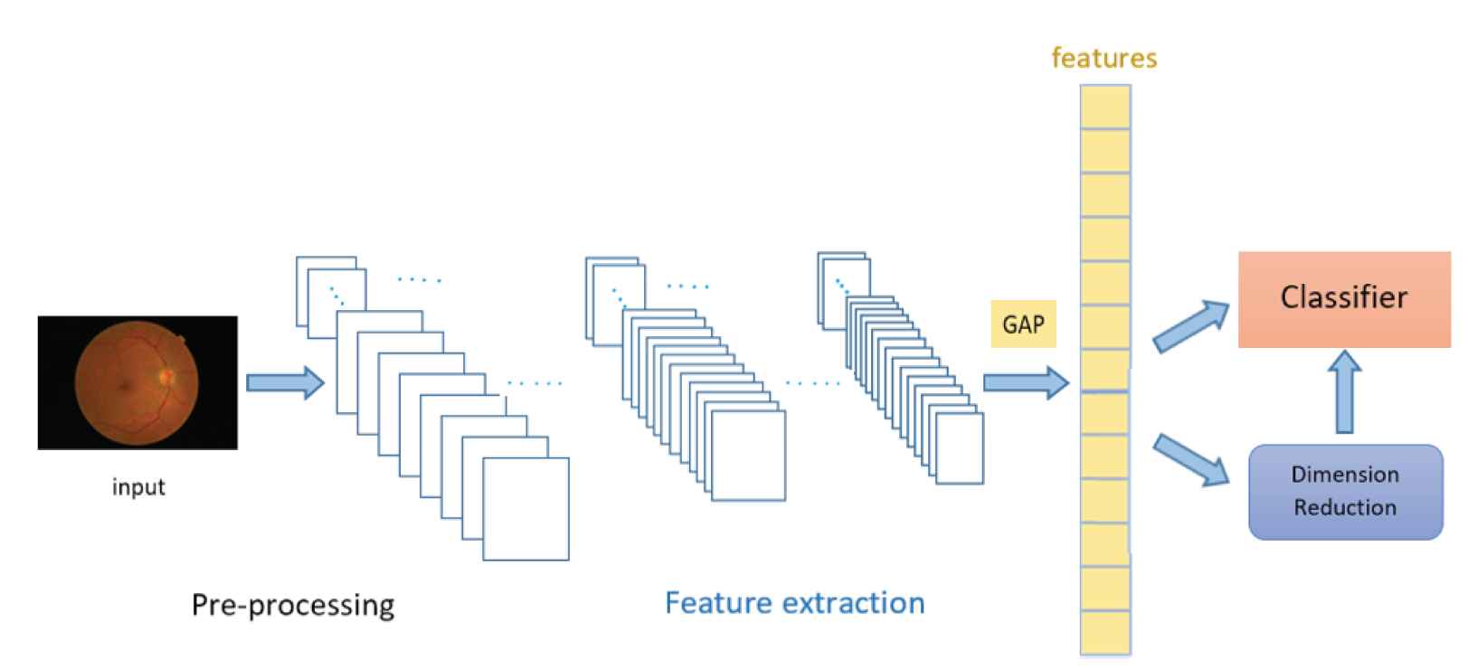
Pipeline of the proposed model.
4. EXPERIMENTAL RESULTS AND DISCUSSION
4.1. Dataset and Preprocessing
In this study, the Messidor-2 dataset [60,61] was used. This dataset includes DR examinations, consisting of macula-centered eye fundus images. Detailed information about the dataset is available on the website given in the acknowledgments section. The Messidor-2 dataset contains 1,748 images and the adjudicated grade levels are: no-DR, mild, moderate, severe, and proliferative DR. Seven images are excluded because of their poor image quality.
Categorization of the fundus images was carried out, following international clinical DR and macular edema disease severity scales (PIRC and PIMEC, respectively). The class name NRDR stands for nonreferable DR. NRDR considers the cases with no DR and mild DR The second class name RDR stands for referable DR. RDR considers the cases with moderate (or worse) DR. This classification has recently been used in DR studies [4].
Table 2 gives the distribution of labeled data. There are 1,286 images in the NRDR class and 455 images in the RDR class. Several pre-processing methods were applied to the images before feeding them into the model. The images were scaled down to an image size of 1200 × 960, in terms of width and height. Image pixel values were converted from [0, 255] to [0, 1] in the RGB (red, green, blue) channels.
| Label | Class | Number |
|---|---|---|
| 0 | NRDR | 1286 |
| 1 | RDR | 455 |
The distribution of relabeled data.
4.2. Experiments
In this study, 1,741 retinal images with a resolution of 1200 × 960 pixels were used in Png and JPG formats. 80% of images were used for training and the remaining images were used for testing. Preprocessed images were fed into the In-centionV3 model, which comprised 10 mixed layers. Features were extracted from the mixed3 layer, which is one of the initial layers of InceptionV3, and frozen weights (layers without layer-wise tuning) were used. Features from the mixed3 layer gave us maximum classification accuracy with applied machine learning algorithms. The GAP operation was applied to the extracted features. GAP helps to decrease overfitting by reducing the total number of parameters in a model and summarizes the presence of features in an image. GAP averages values in the entire feature map and finds a single value for each. A tensor with dimensions h(height) × w(width) × d(depth) is reduced in size to 1 × 1 × d when applying GAP. Features from the GAP outputs are then used directly by the classifiers.
Calibration can make models better predictors, especially for nonlinear machine learning algorithms, which do not directly return probabilistic predictions; rather, they use approximations in classification problems. In this study, the predicted probabilities of different methods were calibrated with the “CalibratedClassifierCV” library in Scikit learn. CalibratedClassifierCV is fitted and calibrated on training data using k-fold cross-validation in the related method, this calibration set is then used in making predictions. In the study by Niculescu-Mizil and Caruana [62], empirical results showed that when calibration is applied, random forests, boosted trees, and SVMs predict better. According to our experimental results, all methods benefit from calibration. Several hyperparameters in the methods were tuned to prevent overfitting or poor performance using the grid search method.
For XGBoost, grid search is carried out for a number of estimators between 100 and 500, for a learning rate between 0.001 and 0.300, and for a maximum depth between 3 and 6. The maximum accuracy is obtained when the parameter combination is: number of estimators = 400; learning rate = 0.1; maximum depth = 4.
For random forest and extra trees classifiers, the number of estimators is searched between 100 and 500. The default number gives the maximum accuracy for random forest. For extra trees, when the number of estimators equals 300, maximum accuracy is obtained. For bagged decision trees, a grid search is carried out for a number of estimators between 10 and 50.
For linear SVC, the maximum iteration number is searched between 1,000 and 11,000. For SVC, the probability parameter is chosen as “True” which enables the classifier to make probability estimates. Available kernel parameters (linear, poly, rbf, sigmoid) and degree (between 3 and 10) are searched. The maximum accuracy is obtained when the parameter combination is probability = True, kernel = poly, degree = 8.
For logistic regression, the maximum iteration number is searched between 100 and 1,200. Available solver parameters (newton-cg; lbfgs, liblinear, sag, saga) are also searched. The default solver, namely lbfgs, gives maximum accuracy. For MLP, hidden layer size and number of neurons in each hidden layer are searched. The learning rate is made “adaptive” and maximum accuracy is obtained when the parameter combination is hidden layer size = 2, number of neurons in each hidden layer = 512.
For dimensionality reduction algorithms, a sufficient number of components in explaining variance is searched.
We chose CalibratedClassifierCV parameters as such: cross-validation value as 5 and method as isotonic. Models are trained on Python 3.7 and scikit learn 0.23.1. Table 3 gives the evaluation results and parameters (except default values) of the methods. Default parameter values are available from the scikit learn [63] and XGBoost official websites, given in the acknowledgments.
| Method | Parameters | Accuracy (%) | AUC (%) |
|---|---|---|---|
| XGBoost | (n_estimators = 400, lr = 0:1, max depth = 4) | 91.40 | 93.55 |
| Random Forest | (n_estimators = 100) | 89.68 | 88.23 |
| ExtraTrees | (n_estimators = 300) | 89.68 | 88.95 |
| Bagged Decision Trees | (n_estimators = 20, be = decisiontree) | 89.40 | 86.63 |
| Linear SVC | (max_iter = 10000) | 89.11 | 91.15 |
| SVC | (probability = True, kernel = poly, degree = 8) | 87.97 | 89.58 |
| Logistic Regression | (max_iter = 10000) | 87.39 | 89.58 |
| MLP | (hidden_layer_sizes = (512,512); lr = adaptive) | 86.53 | 87.49 |
| SVD + XGBoost | (n_f eatures = 19) | 87.10 | 87.91 |
| PCA + XGBoost | (n_f eatures = 19) | 86.24 | 88.38 |
| Kernel PCA + XGBoost | (n_f eatures = 19) | 86.24 | 88.96 |
| Incremental PCA + XGBoost | (n_f eatures = 19) | 85.95 | 88.11 |
lr =learning rate, be =base estimator.
Evaluation results of methods in detecting RDR.
According to the results, the performance of ensemble-based methods is better than the other machine learning methods. XGBoost gives the maximum accuracy, with 91.40%. Random forest and extra trees provide equal accuracy (89.68%) followed by bagging classifier. Linear SVC's (similar to SVC with a linear kernel parameter but implementation is based on liblinear rather than lib-svm) performance is better than SVC: 89.11% and 87.97%, respectively. The performance of logistic regression is close to SVC. Lastly, MLP gives the lowest accuracy of 86.53%.
Tree boosting algorithms are very effective and widely used machine learning methods. XGBoost, as one of the widely used boosting algorithms, enables researchers to achieve a state of the art results on many machine learning problems. In our study, XGBoost outperforms in NRDR vs. RDR classification.
To analyze each case (NRDR, RDR), we presented the confusion matrix of the best classifier, the XGBoost algorithm. For NRDR cases, the XGBoost algorithm classified 268 out of 280 observations correctly, while 51 out of 69 RDR observations were correctly classified. In the confusion matrix given in Figure 3, it can be seen that the misclassification error for RDR cases was greater compared to NRDR cases. This could be due to the number of RDR images being significantly lower than the NRDR cases, which affects the proposed model's detection performance.
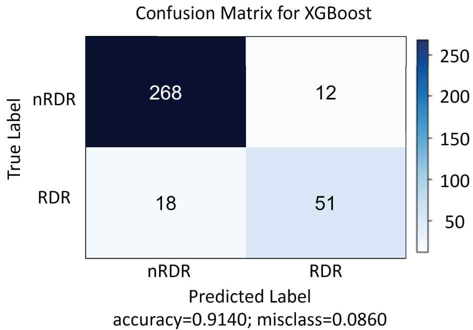
Confusion matrix for XGBoost.
As mentioned before, ensemble learning methods are useful when the training dataset is small, like the Messidor-2 dataset, because they decrease the risk of choosing a weak classifier over individual classifiers. These methods try to improve generalizability or robustness over a single estimator. According to the results, ensemble methods performed better than different SVM, logistic regression, and MLP algorithms.
Summarized features obtained from GAP are reduced with dimensionality reduction algorithms. The number of features is reduced from 768 to 19 for each image. These 19 features explain 95% of the variance for PCA. XGBoost gives an accuracy of 87.10% with truncated SVD; 86.24% with both PCA and kernel PCA; 85.95% with incremental PCA.
Moreover, we built an eight-layer deep CNN model inspired by the AlexNet architecture, one of the most influential papers published in computer vision. The model is comprised five convolutional layers, followed by three fully connected layers. The structure of convolutional layers in our model is the same as AlexNet's convolutional layers, except we used fewer nodes in fully connected layers. Also, we used data augmentation techniques and dropout to prevent overfitting. We trained the model from scratch through 150 epochs with a batch size of 32. Our network architecture has approximately 23 million parameters, in contrast to 60 million parameters reported in the AlexNet paper [64]. The model gives an approximate accuracy of 75%. Considering the developed deep CNN model's performance, in terms of the number of parameters to be trained, training time, and accuracy, our proposed model offers superior performance.
This study shows that when the dataset size is small, machine learning methods with a transfer learning approach give satisfactory results, even without layer-wise tuning.
5. CONCLUSION
The present study offers a model for automated detection of DR in retinal images using the representational power of deep CNN and machine learning methods. The proposed model is based on preprocessing, feature extraction, and classification steps. The main concern was to reduce the complexity and training time of the model while achieving high performance. A pretrained network is used to extract features from images without fine-tuning weights. The extracted features are classified by several machine learning algorithms. Moreover, summarized features are obtained by several dimensionality reduction algorithms. Experiments show that the proposed model yields competitive results, compared with other models trained on the same dataset.
Training the proposed model requires a small number of images, which is valuable, when considering the lack of labeled DR image datasets. The results provide researchers with a performance comparison for different machine learning algorithms.
Our model can also be helpful to ophthalmologists, in diagnosing DR grade.
CONFLICTS OF INTREEST
The authors declare no conflict of interest.
AUTHORS' CONTRIBUTIONS
The authors designed the study commonly. Omer Faruk Gurcan was the primary researcher and responsible for the methodology and experiments. Onur Dogan led the writing of the paper and designed the paper structure. Omer Faruk Beyca was the supervision of the research and responsible for review and editing. All authors have read, revised and approved the final manuscript.
ACKNOWLEDGMENTS
The Messidor program partners kindly provide Messidor-2 dataset (see http://www.adcis.net/en/third-party/messidor/ and http://www.adcis.net/en/thirdparty/messidor2/).
We thank scikit learn and XGBoost developers (https://scikitlearn.org, xgboost.readthedocs.io/)
REFERENCES
Cite this article
TY  - JOUR
AU  - Omer Faruk Gurcan
AU  - Omer Faruk Beyca
AU  - Onur Dogan
PY  - 2021
DA  - 2021/03/22
TI  - A Comprehensive Study of Machine Learning Methods on Diabetic Retinopathy Classification
JO  - International Journal of Computational Intelligence Systems
SP  - 1132
EP  - 1141
VL  - 14
IS  - 1
SN  - 1875-6883
UR  - https://doi.org/10.2991/ijcis.d.210316.001
DO  - 10.2991/ijcis.d.210316.001
ID  - Gurcan2021
ER  -