
Applying Metaheuristic for Time-Dependent Traveling Salesman Problem in Postdisaster
- DOI
- 10.2991/ijcis.d.210226.001How to use a DOI?
- Keywords
- TDTSP; TDTSP-PD; MA; GA; GRASP; VNS
- Abstract
The Time-Dependent Traveling Salesman Problem (TDTSP) is a generalization of the Traveling Salesman Problem (TSP) and Traveling Repairman Problem (TRP). In the TSP and TRP, the travel time to travel is assumed to be constant. However, in practice, the travel times vary according to several factors that naturally depend on the time of day. Therefore, the TDTSP is closer to several real practical situations than the TSP. In this paper, we introduce a new variant of the TDTSP, that is, the Time-Dependent Traveling Salesman Problem in Postdisaster (TDTSP-PD). In the problem, the travel costs need to be added debris removal times after a disaster occurs. To solve the TDTSP-PD, we present an effective population-based algorithm that combines the diversification power of the Genetic Algorithm (GA) and the intensification strength of Local Search (LS). Therefore, our metaheuristic algorithm maintains a balance between diversification and intensification. The results of the experimental simulation are compared with the well-known and successful metaheuristic algorithms. These results show that the proposed algorithm reaches better solutions in many cases.
- Copyright
- © 2021 The Authors. Published by Atlantis Press B.V.
- Open Access
- This is an open access article distributed under the CC BY-NC 4.0 license (http://creativecommons.org/licenses/by-nc/4.0/).
1. INTRODUCTION
1.1. Definition
The problem is a generalization case of the Time-Dependent Traveling Salesman Problem (TDTSP), and at least as hard as the TDTSP. Therefore, it is also NP-hard problem. After that, we define the problem as follows:
Consider a complete graph
The Time-Dependent Traveling Salesman Problem in Postdisaster (TDTSP-PD) is the problem of finding a tour
1.2. Motivation
In recent years, the number of disasters that occur every year are 396. As a result, they affect about 95 million people without essential materials [1]. Therefore, timely delivery of necessary materials, as well as efficient clearing of debris, are related to effective, customer-oriented routing for vehicles. As we know, disasters destroy the infrastructure in cities that cause massive amounts of debris. There are different debris types, such as construction, vegetative, hazardous waste, white goods, freshwater, etc. [1]. Several studies on debris removal have been published in the literature, and they aim at the recovery phase of the disaster that makes the complete removal of debris. However, debris becomes a big issue in the response phase when roads completely or partially are blocked in relief logistics. Our goal is to reach destructed areas as soon as possible, while debris removal complete clearance is impossible because it takes several months to complete. Therefore, a sweeping operation can be deployed so that debris is moved aside and enough space for vehicles to pass.
The classic TDTSP [2–6] is a general variant of the Traveling Salesman Problem (TSP) [7] and Traveling Repairman Problem (TRP) [8,9]. In the TSP and TRP, the travel time to travel is assumed to be constant. However, in practice, the travel times vary according to several factors that naturally depend on the time of day. Therefore, the TDTSP is more practical than the TSP and TRP. The TDTSP has many practical applications in scheduling time-dependent tasks [10–12], scheduling manufacturing system [6], network [13–15], timetables for university [16], schedules vehicles [16], and riding of amusement park attractions [17].
In the TDTSP [3–6], travel time function is defined in normal conditions. However, in disaster situations, travel costs need to be added to debris removal times. The novelty of the problem is to consider an extra effort. This extra effort is an additional time to sweep the debris and make enough space for vehicles. Hence, the TDTSP-PD problem is a single-vehicle routing problem that differs from the classic TDTSP in an important characteristic that is to use the blocked edges. Therefore, the vehicle must spend some extra time to unblock these edges. We can also understand this extra time as a fixed cost defined for edges.
Figure 1 describes an example of the TDTSP-PD. Dashed lines depict the blocked edges. The cost on each edge is the traveling time and debris removal time of the blocked edge. In Figure 1, a couple of values (2, 4) on edge (1, 2) mean that the traveling time from node 1 to 2 is 2 and its debris removal time is 4. For instance, a tour includes nodes 1-2-3-4-1. In this solution, the arrival time to node 2 is 6 (= 2 + 4), to node 3 is 10 (= 6 + 4), to node 4 is 20 (= 10 + 3 + 7), and to return node 1 is 24 (= 20 + 4). Therefore, the total cost is 24.
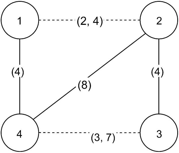
Example of Time-Dependent Traveling Salesman Problem in Postdisaster (TDTSP-PD).
1.3. Literature Review
Though the TDTSP-PD is a natural extension of the classic TDTSP-PD, no publication can be found in the literature. After that, we describe several works to solve the TDTSP in the current. Some formulations for the TDTSP is described in [5]. In Picard et al. [10], Wiel et al. [19], and Bigras et al. [18], the travel time between any two positions depends on the period time of the day. Another variant of the problem is the Time-Dependent Vehicle Routing Problem (TDVRP) in [13,20], where a whole fleet must be routed instead of a single-vehicle.
The TDTSP is NP-hard because it is more challenging than the TSP and TRP [13]. In the TSP, the optimal solutions for large instances [21] are found at a reasonable amount of time. Simultaneously, the exact algorithm [4] can solve only the TDTSP-instances with a few dozen customers. In the TSP, small changes in the structure of a metric space only affect local TSP structure changes. However, this can cause highly nonlocal changes in the structure of the TDTSP problem.
The direct works to the classic TDTSP provided in [2–6] are divided into two categories: 1) The exact algorithms [3,4,19,22] solve exactly instances with small sizes; 2) Several heuristic or metaheuristic algorithms [2,5,11,18,22,23] can produce good solutions fast for large instances. Moreover, some variants of the classic TDTSP [24,25] are known as the TDTSP Time Windows. The above algorithms are the state-of-the-art algorithms for the variants of the TDTSP. However, repairing times for broken roads and debris removal are not mentioned in these problems, and their corresponding algorithms are not easy to be adapted directly to the TDTSP-PD.
Related to the study on postdisaster road clearance and debris removal, Sahin et al. introduce the Debris Removal in the Response Phase problem that requests to reach a set of affected areas as soon as possible by traveling blocked roads due to debris [26]. The problem also considers an extra effort. This extra effort is an additional time to sweep the debris and makes space for vehicles. They developed mathematical models and heuristics to minimize the time to visit critical nodes. This objective is the same as minimizing the maximum latency. Another study related to debris removal is described in [27]. They propose mathematical models and heuristics to minimize 1) minimizing the maximum latency and 2) the total latency of the critical nodes. The experimental results show that their algorithm [26] obtains better solutions than Sahin et al. However, every time the salesman travels the same blocked edge in two problems, the debris removal time is added to the objective function. Thus, there is an over-calculation of the objective value. The TDTSP-PD problem is different from two above problems in four aspects: 1) the travel time to travel in [26,27] is a constant while in our problem it changes drastically that depends on certain time of the day; 2) the debris removal time in our problem does not recalculated on the same edges. Therefore, it does not cause a sub-optimal solution, especially when the number of blocked edges is high; 3) we prefer to minimize the arrival time instead of minimizing maximum latency and total latency; 4) in [26,27], they divide nodes into two types: critical and noncritical nodes. The feasible solution must visit critical nodes, while noncritical ones can be bypassed. Conversely, in the TDTSP-PD problem, all nodes are considered as critical nodes.
1.4. Our Novelties and Contributions
Currently, no work is published for the TDTSP-PD in literature. Our algorithm is the first metaheuristic to solve the problem. Conversely, several works for the TDTSP can be found in the literature. However, comparisons with the results in [6,12,18,22,26] would be meaningless because they were the algorithms a decade ago. In Ban [28] also show that their algorithm is much better than the algorithms in [6,12,18,22,23]. For this reason, we only choose the algorithms [3,28] for the TDTSP as a baseline in our research.
The success of a metaheuristic algorithm depends on the balance between intensification and diversification strategies. The constraint programming approach of Melgarejo [3] takes much time to find a good solution due to memory limits. On the other hand, the metaheuristic in [28] may implement a strong intensification strategy. However, its diversification cannot be sufficient. Therefore, it may get stuck into local optima. In this paper, we proposed the algorithm to overcome the above drawbacks. The main contributions of this work can be summarized as follows:
From the algorithmic perspective, a good metaheuristic must ensure the balance between diversification and intensification. To the best of our knowledge, the work is the first population-based algorithm for the TDTSP-PD and its variants in the literature. To solve this challenging problem, we present the Memetic Algorithm (MA) for the TDTSP-PD. The MA [29] is a powerful population-based framework that balances the diversification of the Genetic Algorithm (GA) [30] and the intensification of Variable Neighborhood Search (VNS) [31].
From the computational perspective, extensive numerical experiments on benchmark instances show the proposed algorithm's efficiency. Moreover, our algorithm reaches better solutions than the-state-of-art algorithms.
The rest of this paper is organized as follows. Section 2 presents the proposed algorithm. Computational evaluations are reported in Section 3. Sections 4 and 5 discuss and conclude the paper, respectively.
2. THE PROPOSED ALGORITHM
In this paper, an efficient metaheuristic proposed brings together the components of GA [30] and VNS [31]. We describe GA and VNS, respectively.
The GA [30] is an evolutionary technique using the survival of the fitness idea. One encodes possible model behaviors into “genes.” After each generation, the parents are allowed to mate and breed based on their fitness. In the process of mating, crossovers and mutations occur. The current population is discarded, and its offspring forms the next generation.
The VNS is described in [31]. It is divided into two main components: The shaking and local search (LS). In the first, shaking implements the move to a random solution. The second consists of applying a LS to the solution and selecting the best one in a neighborhood set.
The MA algorithm for the TDTSP-PD is summarized in Algorithm 1. In the first step, the proposed algorithm generates an initial population. The algorithm then improves it by the VNS in the second step. In the last step, each iteration then implements a crossover and a local optimization. Specifically, the crossover selects and combines two randomly parent solutions to create an offspring. The LS then improves offspring.
Algorithm 1. The proposed algorithm
Input: v1, V, Ni(T)
Output: the best-found solution
1. {Step 1: Generating population}
2. P
3. {Step 2: VNS}
4. for
5. Ti
6. endfor
7. {Step 3: Crossover+VNS}
8. while (stop condition is not met) do
9. Select parent TP, TM from P
10. TC = Crossover(TP, TM);
11. TC = VNS(TC);
12. {Updating the population}
13. P = Elitism-Selection(TC, P);
14. endwhile
15.
16. return
Finally, an update of the population is implemented. The algorithm finishes after a fixed number of generations.
To make the algorithm's structure more detail, a flowchart of the MA algorithm is described in Figure 2. The algorithmic steps are described in the following sections.
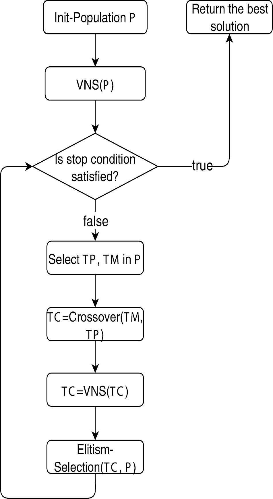
The flowchart of the Memetic Algorithm (MA) algorithm.
2.1. Encoding and Evaluation
The simple encoding is used, in which a tour is represented as a list of n vertices
2.2. Generating Population
We use two methods to create individuals. In the first method, we pick a number randomly between one and one hundred. If the number is less than β, the individual will be created randomly. Conversely, it will be the output result of the Greedy Randomized Adaptive Search Procedure (GRASP) [32]. Two methods are used for initialization to generate enough diversity of the population. The size of the population SP is the parameter determined in the experiments. Details of steps are given in Algorithm 2.
Algorithm 2. Init-Population
Input: v1, V,
Output: An initial solution T.
1. While
2.
3. type = rand(1);
4. if (Type ≤ β) then
5. while |T| < n do
6. Select randomly vertex
7.
8. endwhile
9. else
10. while
11. {
12. Create RCL that includes
13. Select randomly vertex
14.
15. endwhile
16. endif
17.
18. return
2.3. Variable Neighborhood Search
2.3.1. Neighborhoods
We use neighborhoods widely applied in the literature to explore this problem's solution space [7]. Assume that T, and n are a tour, and its size, respectively. We describe more details about five neighborhoods (kmax = 5) as follows:
shift (N1) relocates a vertex to another position in T.
swap-adjacent (N2) tries to swap each pair of adjacent vertices in T.
swap (N3) tries to swap the positions of each pair of vertices in T.
2-opt (N4) removes each pair of edges from the tour and reconnects them.
Or-opt (N5) reallocates three adjacent vertices to another position of T.
The VNS executes neighborhood procedures in turn and shaking techniques. At each iteration, the best neighboring solution is chosen from neighboring solutions generated from a neighborhood procedure. If it is better than the current best one, the procedure is repeated. Otherwise, the search goes to the next neighborhood procedure. The detail is described in Algorithm 3.
Algorithm 3. VNS
Input:
Output: the best solution
1.
2. T = Variable Neighborhood Decent (VND) (T);
3. while
4.
5.
6. if
7.
8. if
9.
10. endif
11. endif
12. if (
13.
14. else
15.
16. endif
17. endwhile
18. return
2.3.2. Perturbation
The Perturbation mechanism is very important to escape local optima. When the mechanism has too small moves, the search can return to the previously visited solution space. On the other hand, large moves drive the search to undesirable space. To balance the strength of shaking (notation: level ), we propose a new shaking technique based on the original double-bridge technique [33]. The detail is described in Algorithm 5.
Algorithm 4. VND
Input:
Output: the best solution
1.
2. repeat
3. Find the best neighborhood
4. if
5.
6. if
7.
8. endif
9.
10. else
11.
12. endif
13. until
14.
15. return
The fitness function represents the evaluation of individuals. This evaluation function will check the cost of an individual. The less the cost is, the better the individual is.
Algorithm 5. Perturbation
Input:
Output: a new tour
1.
2. while
3.
4.
5. If
6.
7. break;
8. else
9.
10. endif
11. endwhile
12. return
2.4. Selection Operator
The selection phase is when the individuals are selected based on their fitness to mate and produce new offspring. In this work, the simple selection operator is used [34]. A group of number of individuals (NG) with a specified size is selected on a random basis. Then, two individuals that have the best fitness in the group will be chosen. The fitness difference provides selection pressure. Increased selection pressure can be provided by simply increasing the size of the group, as the winners from a larger size will, on average, have higher fitness than the winners of a small size.
2.5. Crossover
Crossover operators are significant as their exploratory force because of their ability to explore solutions over a wider search space area. Crossover is the process that mimics mating between two individuals to produce children. In Otman and Jaafar [35], the crossover operators are classified as follows: 1) The crossover operators focus heavily on the position of certain genes in the parents such as Partially Mapped Crossover (PMX), Cycle Crossover (CX), Position-Based Crossover (POS), etc.; 2) The crossovers create an offspring by selecting genes alternately from the parents while the repetition of genes is abandoned such as Edge Exchange Crossover (EXX), Edge Assembly Crossover (EAX), Heuristic Crossover (HGreX), etc.; 3) The crossovers inherit the order of genes from parent to the offspring such as Sorting Crossover (SC), Merging Crossover (MC), and Uniform Like Crossover (ULX), etc. We found no logical explanation of which one should bring better performance or better overall results. That means there is not the best crossover for all cases. In a pilot study, we found that the algorithm's performance is relatively insensitive to crossover operators. As testing our algorithm on all operators would have been computationally too expensive, we implement our numerical analysis on some selected operators for each type. In this work, the following operators are selected: type 1 (PMX), type 2 (EXX), and type 3 (SC) [35]. Using multiple crossovers makes the population more diverse than using only one crossover. Therefore, it can help the algorithm to prevent being trapped in a local optimum. The detail in this step is given in Algorithm 6.
Algorithm 6. Crossover
Input:
Output: A new child
1. If (type==1) then
{type 1 is chosen}
2. TC = PMX(TP, TM); {PMX is chosen}
3. else if (type==2)
4. {type 2 is chosen}
5. TC = EXX(TP, TM); {EXX is chosen}
6. else if (type==3)
7. {type 3 is chosen}
8. TC = SC(TP, TM); {SC is chosen}
9. endif
10. return TC;
2.6. Updating the New Population
Each new solution generated by the VNS should be have appeared in the population. If it is better than the worst solution in the population, then it replaces the worst one. On the other hand, the population remains unchanged.
2.7. Stop Condition
The last aspect to discuss is the stop criterium of our algorithm. A balance must be made between computation time and efficiency. Here, the algorithm stops if no improvement is found after m loops.
3. EVALUATIONS
Our algorithm is implemented on a Pentium 4 core i7 2.40 GHz processor with 8 GB of RAM. In all experiments, parameters
3.1. Instances
Our datasets are the TDTSP-benchmarks in [36]. Their instances are generated from 255 locations randomly chosen from a list of tours of drivers in Lyon. In this dataset, the number of time steps is 130. At the same time, each duration is 360 seconds. On hundred instances are generated for each problem size from 20 to 100. The duration of each visit is randomly selected in [60, 300] seconds. Due to the traffic jam, they create three travel time functions. In this experiment, 180 instances from 50 to 100 vertices are chosen.
To generate different scenarios in disaster situations, we assumed five levels of earthquake severity (LES), which varies from 1 to 5. Since the level is 1, there is a less severe earthquake. On the other hand, when the level is 5, it yields the highest severe earthquake. The higher and higher severe earthquake is, the more and more broken edges occur. Table 1 illustrates the broken edge ratios (BER) according to the severe earthquake. Repairing times
| LES | #BER |
|---|---|
| 1 | 0%–20% |
| 2 | 20%–40% |
| 3 | 40%–60% |
| 4 | 60%–80% |
| 5 | 80%–100% |
BER, broken edge ratios; LES, levels of earthquake severity.
LES and corresponding BER values.
3.2. Metrics
We define the proposed algorithm's improvement with respect to the upper bound (UB) obtained by the Nearest Neighborhood Search [7]. The Nearest Neighborhood Search is not promising theoretically; however, it yields good enough solutions in practice.
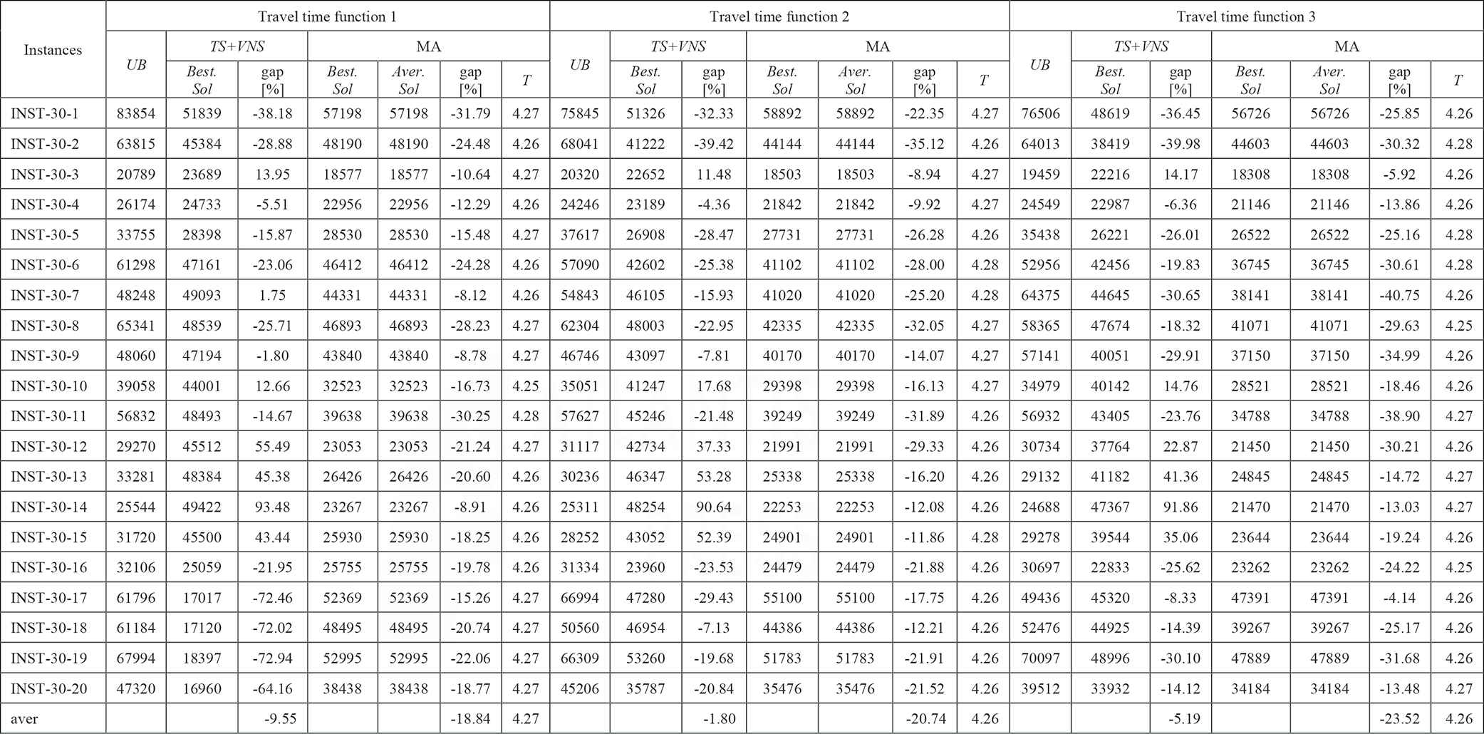
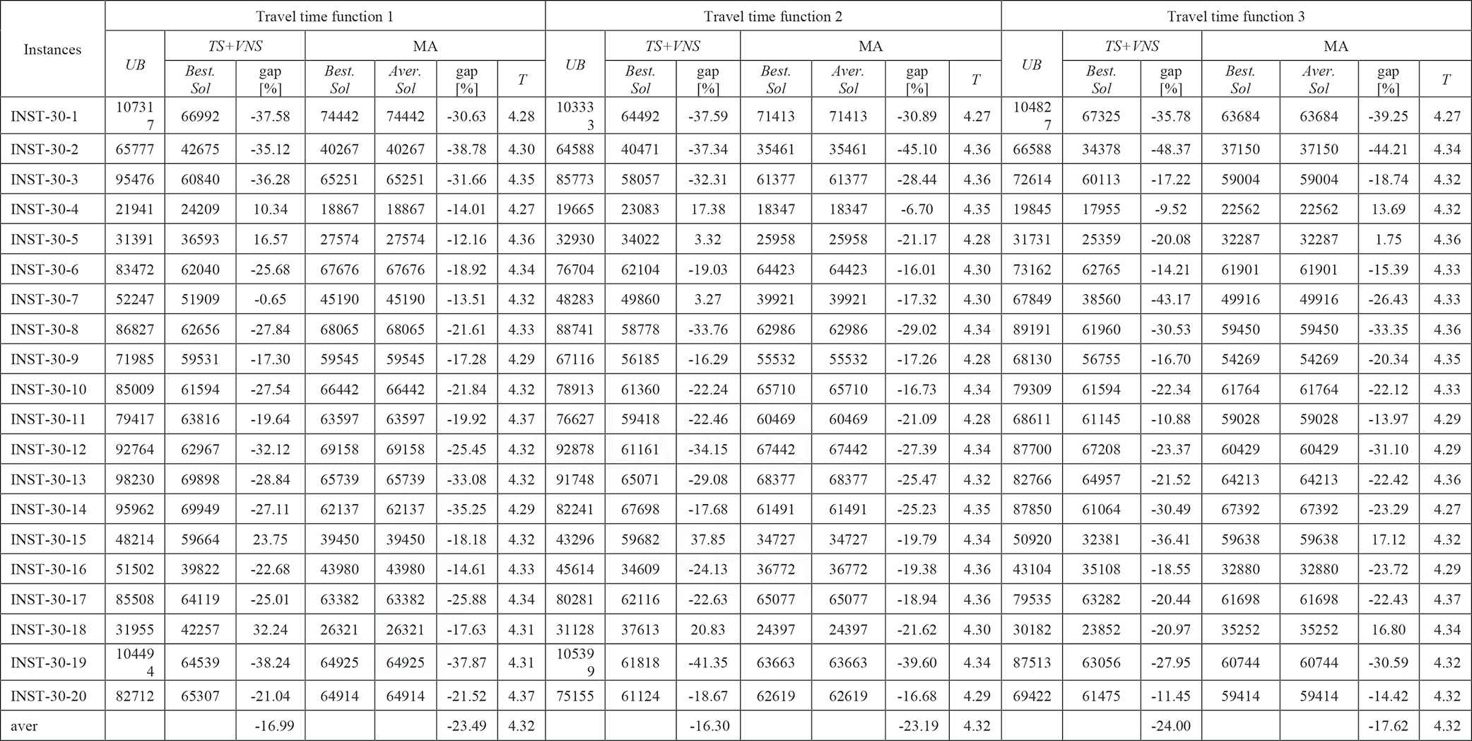
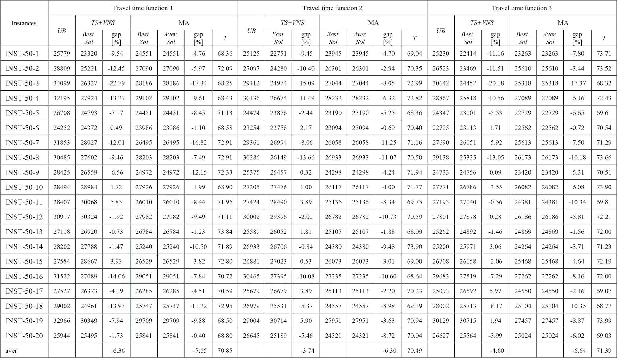
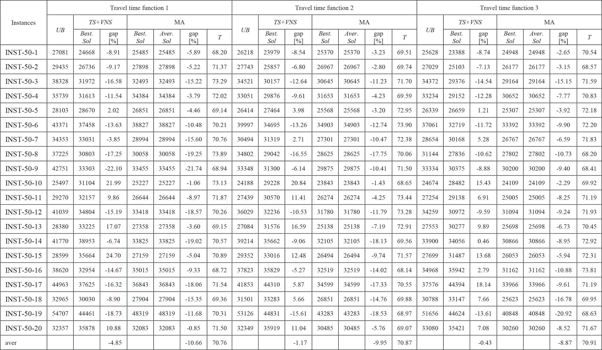
In addition, our solutions are also compared to the optimal or best solutions [3,4,28] for variants though it is not designed to solve them. The proposed algorithm runs on the same instances with the other algorithms. In all Tables, the same or improved results are highlighted in boldface and red, respectively. In addition, OPT, Best.Sol, Aver.Sol, and T correspond to the optimal solution, best solution, average solution, and average time in seconds of ten executions obtained by the proposed algorithm.
3.3. Comparison with UB
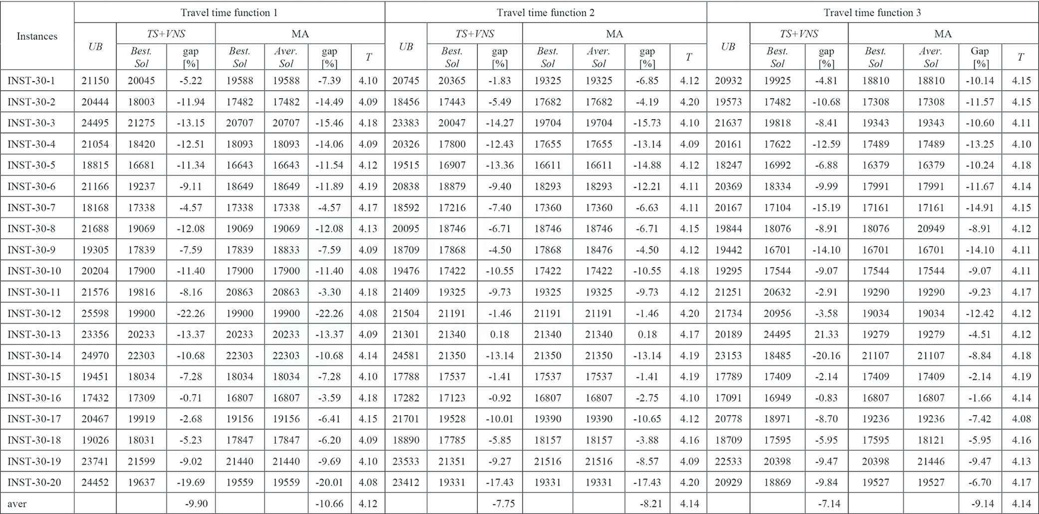
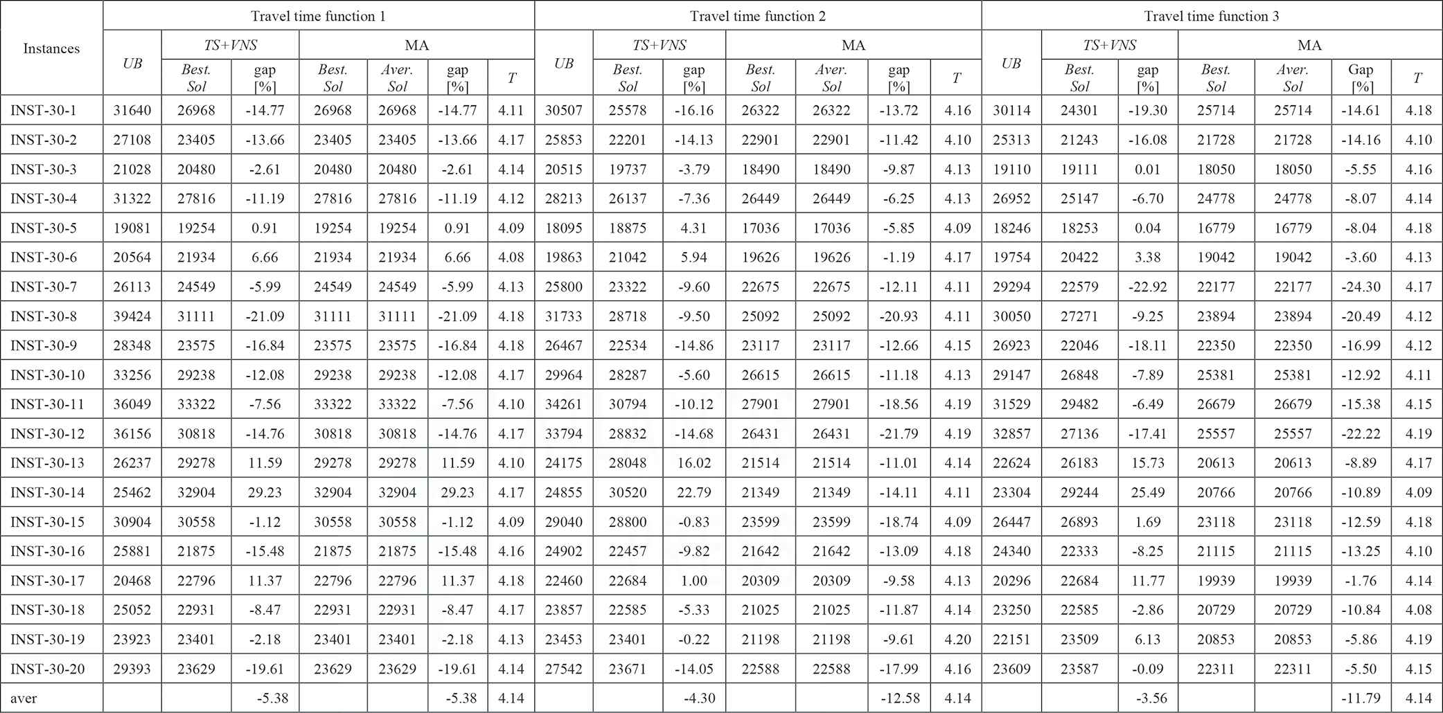
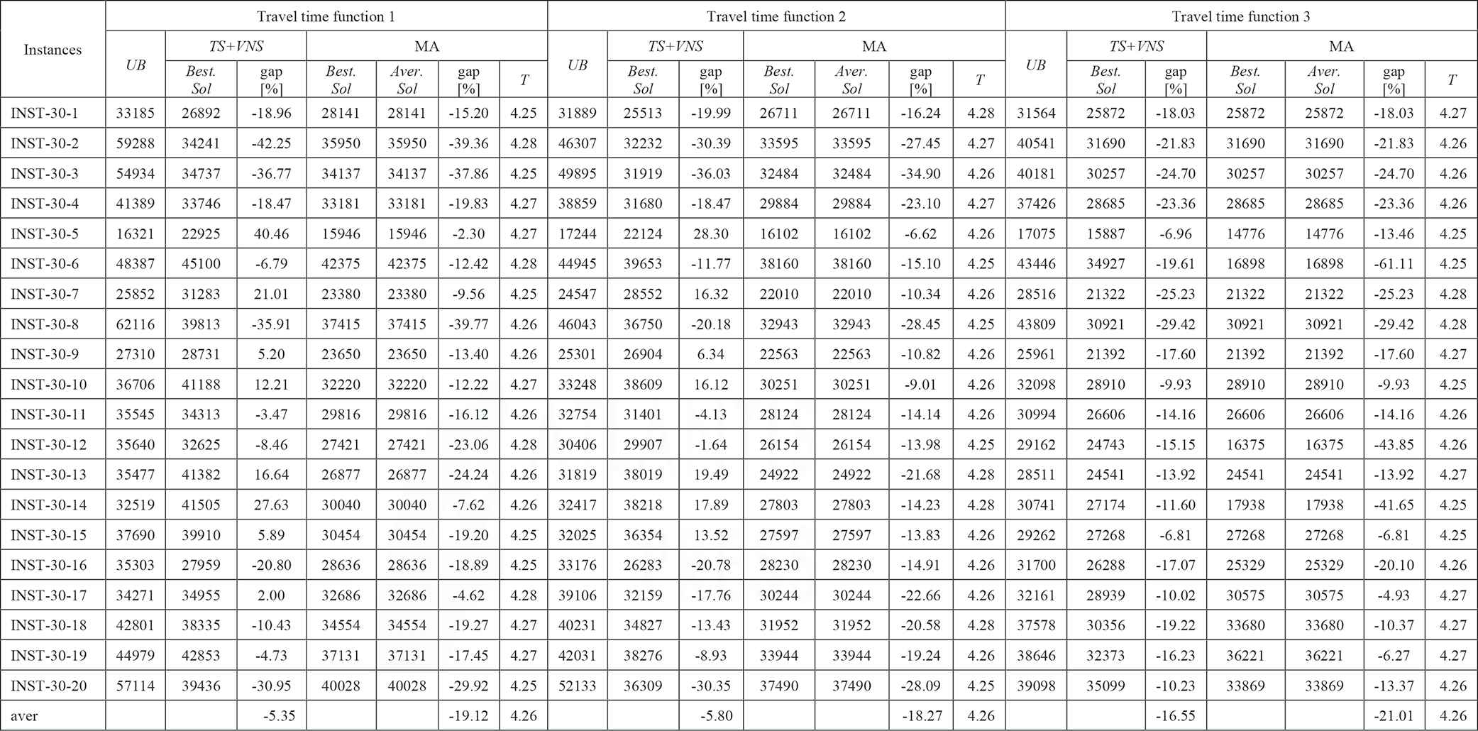
Tables A1–15 compare the results of the proposed algorithm with the UB. The values in Table 2 are the average ones calculated from Tables A1–15 in Appendix.
| Instances | Travel Time Function 1 | Travel Time Function 2 | Travel Time Function 3 | ||||||
|---|---|---|---|---|---|---|---|---|---|
| TS+VNS | MA | TS+VNS | MA | TS+VNS | MA | ||||
| gap [%] | gap [%] | T | gap [%] | gap [%] | T | gap [%] | gap [%] | T | |
| INST-30-x (LES=1) | −9.9 | −10.66 | 4.12 | −7.75 | −8.21 | 4.14 | −7.14 | −9.14 | 4.14 |
| INST-30-x (LES=2) | −5.38 | −5.38 | 4.14 | −4.3 | −12.58 | 4.14 | −3.56 | −11.79 | 4.14 |
| INST-30-x (LES=3) | −5.35 | −19.12 | 4.26 | −5.8 | −18.27 | 4.26 | −16.55 | −21.01 | 4.26 |
| INST-30-x (LES=4) | −9.55 | −18.84 | 4.27 | −1.8 | −20.74 | 4.26 | −5.19 | −23.52 | 4.26 |
| INST-30-x (LES=5) | −16.99 | −23.49 | 4.32 | −16.3 | −23.19 | 4.32 | −24 | −17.62 | 4.32 |
| INST-50-x (LES=1) | −6.36 | −7.65 | 70.85 | −3.74 | −6.3 | 70.49 | −4.6 | −6.64 | 71.39 |
| INST-50-x (LES=2) | −4.85 | −10.66 | 70.76 | −1.17 | −9.95 | 70.87 | −0.43 | −8.87 | 70.91 |
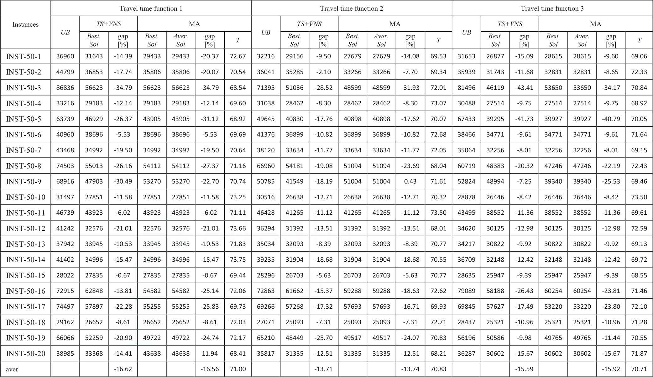
| INST-50-x (LES=3) | −16.62 | −16.56 | 71 | −13.71 | −13.74 | 70.83 | −15.59 | −15.92 | 70.71 |
| INST-50-x (LES=4) | −24.07 | −25.93 | 71.33 | −22.69 | −23.17 | 70.96 | −21 | −21.31 | 71.34 |
| INST-50-x (LES=5) | −28.16 | −29.61 | 70.42 | −25.91 | −27.1 | 71.8 | −26.82 | −28.62 | 70.51 |
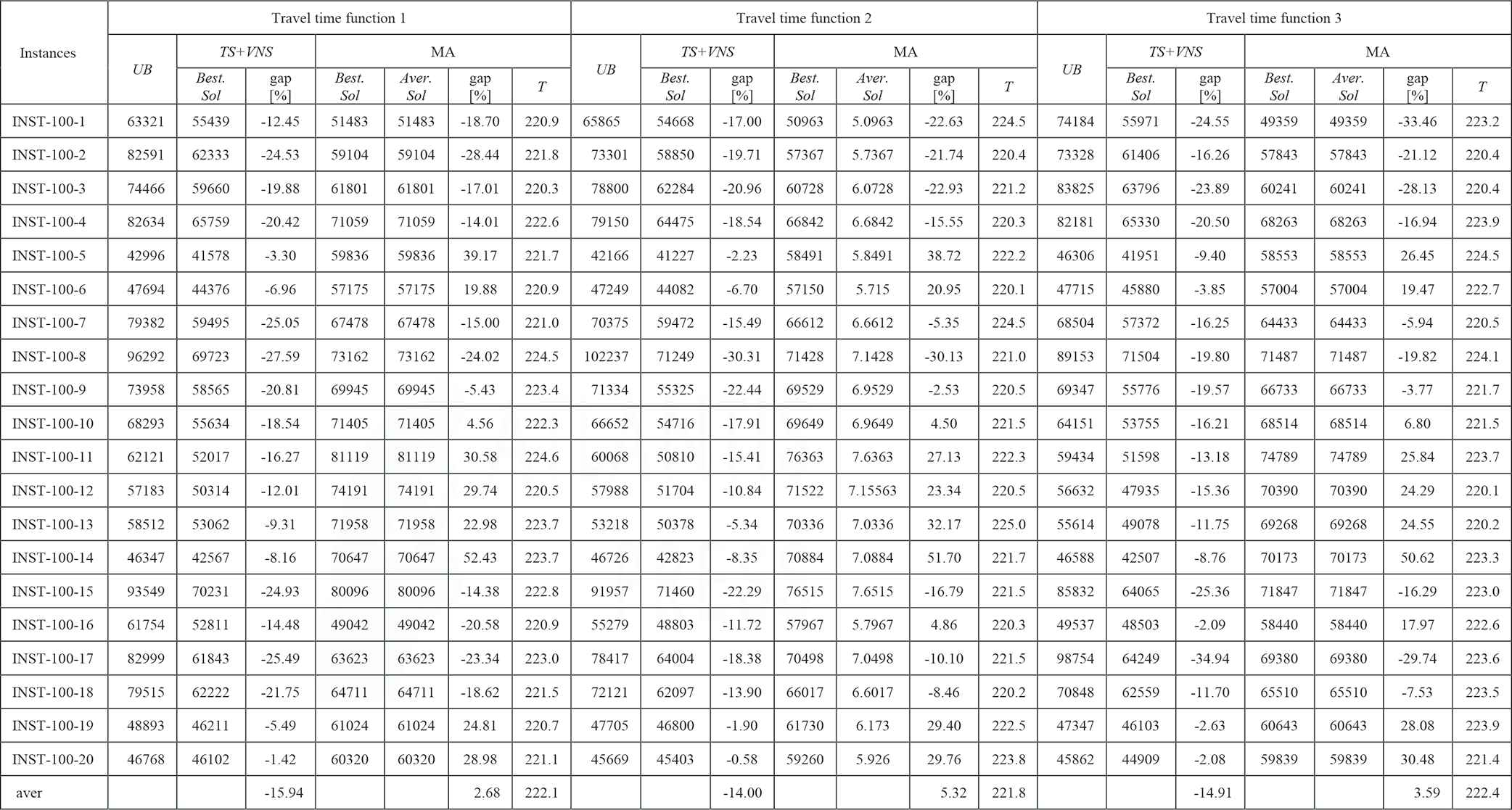
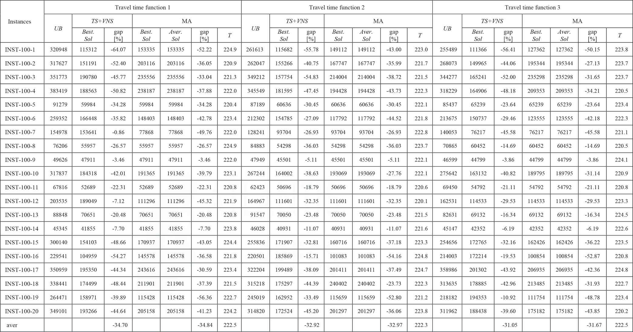
| INST-100-x (LES=1) | −7.27 | −9.12 | 222.2 | −7.09 | −8.23 | 222.6 | −7.72 | −9.12 | 222.6 |
| INST-100-x (LES=2) | −15.94 | 2.68 | 222.1 | −14 | 5.32 | 221.8 | −14.91 | 3.59 | 222.4 |
| INST-100-x (LES=3) | −26.68 | −28.68 | 222.5 | −25.24 | −27.7 | 222.6 | −21.42 | −24.2 | 221.9 |
| INST-100-x (LES=4) | −29.85 | −33.59 | 222.5 | −28.37 | −31.88 | 221.9 | −26.06 | −32.22 | 221.9 |
| INST-100-x (LES=5) | −34.7 | −34.84 | 222.5 | −32.92 | −32.97 | 222.3 | −31.05 | −31.67 | 222.5 |
| Aver | −16.11 | −18.10 | −14.05 | −17.25 | −15.07 | −17.20 | |||
MA, Memetic Algorithm; TDTSP-PD, Time-Dependent Traveling Salesman Problem in Postdisaster; TS, Tabu Search; VNS, Variable Neighborhood Search.
The average experimental results for TDTSP-PD with instances that are proposed by [25].
In Table 2, for each dataset, the average gap between the UB and our best solution varies between −14.05% and −18.10%. Obviously, the improvement is large and significant. These results further indicate the proposed algorithm reaches good solutions fast.
3.4. Comparison the Difference between the Objective Values of the TDTSP and TDTSP-PD
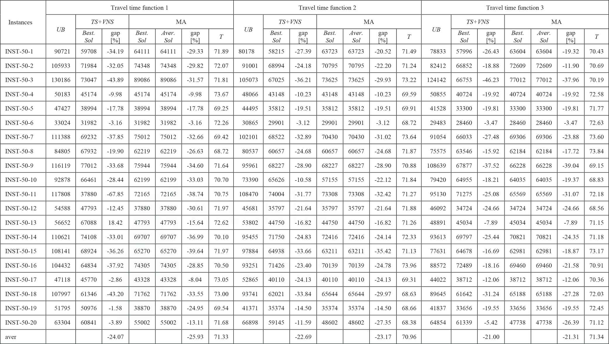
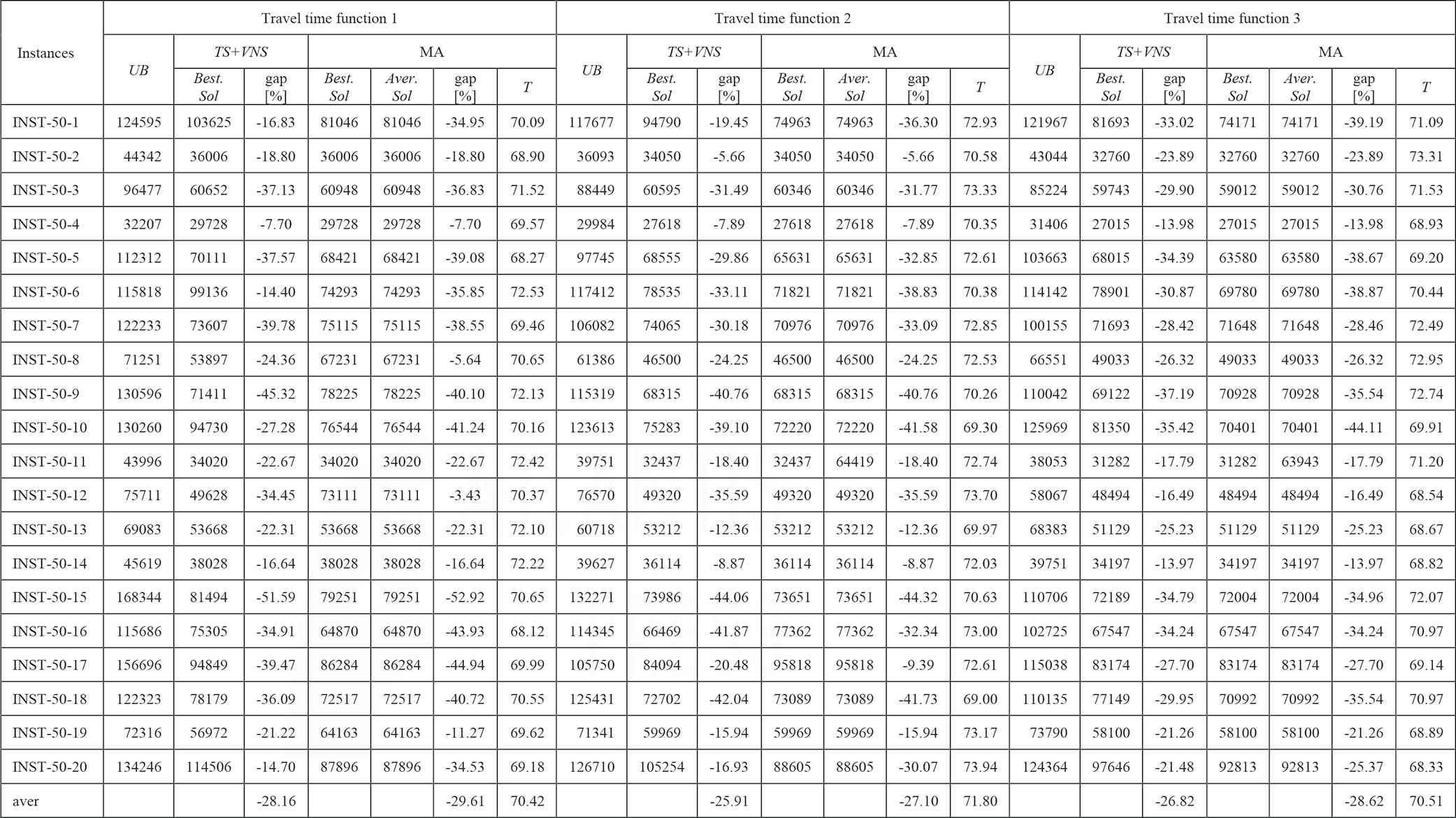
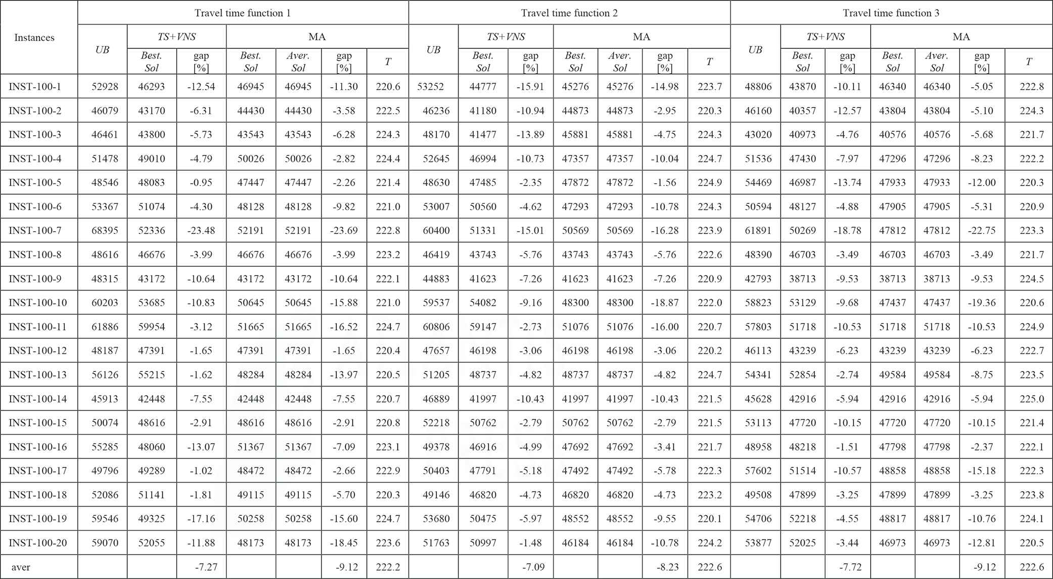
In Tables A1–15 in the Appendix, we also see that the higher and higher the value of LES is, the larger and larger the objective function cost is. It is suitable in practical situations because debris removal time for a high level of earthquake severity consumes more time than the lower level cases.
Table 5 shows the difference between the objective value of the TDTSP and TDTSP-PD with five values of LES. The results show that when LES's value is small (LES = 1), the difference between them is not large because debris removal operation takes a little time to unblocked roads in this case. Conversely, the difference becomes large with the LES's other values (LES = 2, 3, …, 5). It shows that most of the time in these cases is used to clear debris other than travel on the roads.
3.5. Comparison with TS+VNS
Recently, Tabu Search (TS) [28] has been successfully applied to solve the TDTSP. To compare directly with the TS+VNS, we adapt the TS+VNS algorithm for the TDTSP to the TDTSP-PD case. Fortunately, Ban [28] support us to access their code. We also remain the parameter settings unchanged.
In Table 2, the results show that the robustness of the proposed algorithm. More precisely, the average gap between the two algorithms is −2.44%. In 900 instances, our algorithm obtains better solutions in 407 cases and the same solutions in 203 cases (see more detail in Tables A1–15 in the Appendix). To indicate a clear dominance of the proposed algorithm over the TS+VNS, Wilcoxon's test [37] is used. Table 3 shows Wilcoxon signed ranks test results between the TS+VNS and MA in 900 cases. The results indicate that the MA shows a significant improvement over the TS+VNS with a level of significance α = 0.05.
| Problems | R+ | R− | p -value |
|---|---|---|---|
| TDTSP-PD | 109552 | −53299 | <0.0001 |
| TDTSP | 2215 | −474 | <0.0001 |
TDTSP, Time-Dependent Traveling Salesman Problem; TDTSP-PD, Time-Dependent Traveling Salesman Problem in Postdisaster; TS, Tabu Search; VNS, Variable Neighborhood Search.
Wilcoxon signed ranks test results between the TS+VNS and MA for the TDTSP-PD and TDTSP with a level of significance α = 0.05.
To compare their time complexity, three perspectives [23] can be considered as follows:
The theoretical time complexity: The time complexity of the MA mainly spends to explore in VNS. In VNS, the time complexity of the Or neighborhood is not less than those of the other neighborhoods. Assume that, when k is its maximum number of runs in the algorithm, the MA requires
The time complexity by CPU times: Ban [28] support us to access their code. Therefore, two algorithms are run on the same computer languages, platforms, and compilers. It is convenient to compare the running time of them by CPU times. In Table 4, the running time of the proposed algorithm grows moderate compared to the TS+VNS. The result is understandable because a population-based metaheuristic often consumes more time than a single-based one.
The time complexity by function evaluations: For several expensive optimization problems, the function evaluation reflects an algorithm's time complexity. In the TDTSP-PD, the evaluation function is not too expensive when it consumes O(n) time. The fundamental evaluations do not completely dominate the internal workings of the algorithm. However, to help us evaluate two algorithms' time complexity more exactly, the maximum number of fitness function evaluations is also mentioned. We count the maximum number of fitness evaluations such that the MA obtains the best solution. After that, we run the TS+VNS with the same maximum number of fitness evaluations. The results of the TS+VNS still remains unchanged. The TS+VNS cannot find any better solutions in all instances though in many cases it may be run with the additional number of fitness evaluations. The TS+VNS might have a strong search for intensification capacity. Their diversification technique may not be sufficient to bring the search to unexplored search space regions. Therefore, it can get stuck into local optima. The additional number of fitness evaluations does not help it to improve the solution quality. Due to the random nature, our population-based algorithm can explore a more extensive solution space. As a result, the chance of finding the optimal solution is higher.
| Instance | TS+VNS | MA |
|---|---|---|
| INST-30-x | 1.32 | 4.22 |
| INST-50-x | 5.89 | 70.94 |
| INST-100-x | 38.51 | 222.28 |
| Aver | 15.24 | 99.14 |
MA, Memetic Algorithm; TDTSP-PD, Time-Dependent Traveling Salesman Problem in Postdisaster; TS, Tabu Search; VNS, Variable Neighborhood Search.
Comparison for the running time by seconds between TS+VNS and MA for the TDTSP-PD.
| Instances | Travel Time Function 1 | Travel Time Function 2 | Travel Time Function 3 |
|---|---|---|---|
| diff [%] | diff [%] | diff [%] | |
| INST-50-x (LES=1) | 16.06 | 14.24 | 70.49 |
| INST-50-x (LES=2) | 37.12 | 37.12 | 70.76 |
| INST-50-x (LES=3) | 75.28 | 71.00 | 68.11 |
| INST-50-x (LES=4) | 160.44 | 151.33 | 153.71 |
| INST-50-x (LES=5) | 184.22 | 176.50 | 174.14 |
| INST-100-x (LES=1) | 22.80 | 24.83 | 222.6 |
| INST-100-x (LES=2) | 68.85 | 74.08 | 76.64 |
| INST-100-x (LES=3) | 100.63 | 105.76 | 111.50 |
| INST-100-x (LES=4) | 157.90 | 154.80 | 155.41 |
| INST-100-x (LES=5) | 256.84 | 243.78 | 252.63 |
MA, Memetic Algorithm; TDTSP-PD, Time-Dependent Traveling Salesman Problem in Postdisaster; TS, Tabu Search; VNS, Variable Neighborhood Search.
The difference objective value between TDTSP-PD and TDTSP with the values of LES.
In summary, on average, the MA consumes more time than the TS+VNS. Nevertheless, the fact that their running time difference is quite moderate. In addition, the TS+VNS does not improve solution quality though the additional number of fitness evaluations may be allowed. In that case, we can still say that our MA is beneficial.
3.6. Experimental Results on TDTSP Instances
From Tables 6 and 7, we know that most algorithms are developed for a specific variant that does not apply to the other variants. Our algorithm still runs well to the TDTSP, although it was not designed for solving it. In comparison with the best-known solution in [3,28], our algorithm's solutions obtain better solutions than the Melgarejo's algorithm [3], and Ban's algorithm [28] in many cases. The improvement is significant since it can be observed that our algorithm is capable of finding the new best solutions in 69 instances. To have more clear statistical comparison, the Wilcoxon's test is still used. Table 3 shows that the MA shows a significant improvement over the TS+VNS with a level of significance α = 0.05. However, the proposed algorithm consumes more time compared to Melgarejo's [3] and Ban's algorithm [3,28] (see Table 8).
| Instances | Travel Time Function 1 | Travel Time Function 2 | Travel Time Function 3 | ||||||||||||
|---|---|---|---|---|---|---|---|---|---|---|---|---|---|---|---|
| PAM | BA | MA |
PAM | BA | MA |
PAM | BA | MA |
|||||||
| Best.Sol | Aver.Sol | T | Best.Sol | Aver.Sol | T | Best.Sol | Aver.Sol | T | |||||||
| INST-50-1 | 22795 | 22846 | 22537 | 22537 | 84.05 | 22108 | 22108 | 22010 | 22010 | 83.76 | 21678 | 21718 | 21678 | 21678 | 83.16 |
| INST-50-2 | 23421 | 23713 | 23421 | 23421 | 83.74 | 22661 | 23233 | 22475 | 22475 | 81.14 | 22676 | 22287 | 22108 | 22108 | 81.78 |
| INST-50-3 | 22684 | 22684 | 22431 | 22431 | 80.60 | 21777 | 21777 | 21777 | 21777 | 80.32 | 21382 | 21217 | 21354 | 21354 | 84.99 |
| INST-50-4 | 24396 | 24833 | 24406 | 24406 | 82.63 | 23579 | 23610 | 23553 | 23553 | 83.84 | 22949 | 22976 | 22949 | 22949 | 81.12 |
| INST-50-5 | 20960 | 20960 | 20960 | 20965 | 81.63 | 20877 | 20877 | 20877 | 20877 | 83.36 | 20553 | 20610 | 20658 | 20658 | 83.26 |
| INST-50-6 | 22074 | 22396 | 21966 | 21966 | 82.73 | 21380 | 21795 | 21795 | 21795 | 83.58 | 21276 | 20950 | 21046 | 21046 | 83.02 |
| INST-50-7 | 23241 | 23241 | 23241 | 23126 | 81.99 | 22645 | 22645 | 22650 | 22650 | 83.21 | 22308 | 22371 | 22464 | 22464 | 81.94 |
| INST-50-8 | 23274 | 23274 | 23274 | 23274 | 82.08 | 22558 | 22558 | 22576 | 22576 | 82.10 | 22182 | 22014 | 22005 | 22005 | 80.71 |
| INST-50-9 | 22549 | 22549 | 22549 | 22549 | 80.90 | 22015 | 22015 | 22015 | 22015 | 81.95 | 21669 | 21913 | 21669 | 21669 | 80.13 |
| INST-50-10 | 22556 | 22831 | 22195 | 22195 | 81.28 | 21861 | 22249 | 21655 | 21655 | 84.08 | 21928 | 21427 | 21429 | 21429 | 82.11 |
| INST-50-11 | 23775 | 23893 | 23530 | 23530 | 80.10 | 23015 | 23063 | 22974 | 22974 | 81.59 | 22230 | 22490 | 22357 | 22357 | 80.92 |
| INST-50-12 | 24487 | 24610 | 24035 | 24035 | 84.62 | 23792 | 23969 | 23792 | 23792 | 84.07 | 23568 | 23131 | 23100 | 23100 | 83.63 |
| INST-50-13 | 23432 | 23432 | 23148 | 23148 | 83.27 | 22585 | 22585 | 22578 | 22578 | 83.95 | 22190 | 22121 | 22095 | 22095 | 81.85 |
| INST-50-14 | 23452 | 23678 | 23389 | 23389 | 84.66 | 22677 | 22737 | 22729 | 22729 | 84.26 | 22103 | 22238 | 22211 | 22211 | 84.21 |
| INST-50-15 | 22473 | 22473 | 22829 | 22829 | 80.82 | 21838 | 21838 | 21869 | 21869 | 82.53 | 22057 | 21490 | 21440 | 21440 | 83.67 |
| INST-50-16 | 23538 | 23538 | 23509 | 23509 | 84.61 | 23032 | 23035 | 22962 | 22962 | 83.18 | 22463 | 22461 | 22463 | 22463 | 82.86 |
| INST-50-17 | 24028 | 24100 | 24028 | 23862 | 83.97 | 23273 | 23311 | 23055 | 23055 | 84.75 | 23207 | 22644 | 22753 | 22753 | 80.88 |
| INST-50-18 | 21181 | 21539 | 21181 | 21181 | 82.89 | 20785 | 20785 | 20832 | 20832 | 82.22 | 20681 | 20483 | 20483 | 20483 | 84.79 |
| INST-50-19 | 24477 | 24477 | 24501 | 24501 | 82.20 | 23899 | 23899 | 23821 | 23821 | 80.30 | 23332 | 23274 | 23268 | 23268 | 81.33 |
| INST-50-20 | 22528 | 23170 | 23170 | 23170 | 81.29 | 22180 | 22499 | 22071 | 22071 | 84.33 | 21984 | 21655 | 21691 | 21691 | 84.62 |
| aver | 82.50 | 82.93 | 82.55 | ||||||||||||
MA, Memetic Algorithm; TDTSP, Time-Dependent Traveling Salesman Problem.
The bold values in Table 6 means that our solutions are better or at least as well as the other algorithms (PAM and BA).
The experimental results for TDTSP with INST-50-x instances that are proposed by [25].
| Instances | Travel Time Function 1 | Travel Time Function 2 | Travel Time Function 3 | ||||||||||||
|---|---|---|---|---|---|---|---|---|---|---|---|---|---|---|---|
| PAM | BA | MA |
PAM | BA | MA |
PAM | BA | MA |
|||||||
| Best.Sol | Aver.Sol | T | Best.Sol | Aver.Sol | T | Best.Sol | Aver.Sol | T | |||||||
| INST-100-1 | 39532 | 39249 | 39249 | 39205 | 231.12 | 39336 | 38245 | 37801 | 37801 | 231.38 | 36884 | 36884 | 36431 | 36431 | 230.69 |
| INST-100-2 | 36015 | 36015 | 36015 | 35563 | 231.87 | 35065 | 35143 | 34419 | 34419 | 231.24 | 34793 | 33987 | 34793 | 34793 | 231.09 |
| INST-100-3 | 36807 | 36807 | 36869 | 36869 | 230.44 | 37240 | 35729 | 35330 | 35330 | 232.26 | 37000 | 34477 | 34470 | 34470 | 230.91 |
| INST-100-4 | 39631 | 39631 | 39284 | 39284 | 233.20 | 38954 | 38240 | 38027 | 38027 | 231.14 | 39558 | 37765 | 36811 | 36811 | 230.21 |
| INST-100-5 | 38396 | 37377 | 36757 | 36757 | 230.90 | 35852 | 35852 | 35685 | 35685 | 234.02 | 34580 | 34580 | 35056 | 35056 | 230.53 |
| INST-100-6 | 37957 | 38312 | 37444 | 37444 | 230.23 | 36508 | 36508 | 36163 | 36163 | 234.93 | 34950 | 34950 | 35243 | 35243 | 233.08 |
| INST-100-7 | 41457 | 40371 | 40460 | 40460 | 233.62 | 37971 | 39081 | 38425 | 38425 | 230.15 | 36395 | 36395 | 37217 | 37217 | 234.70 |
| INST-100-8 | 39302 | 39302 | 39847 | 39847 | 231.74 | 39325 | 39257 | 38085 | 38085 | 232.68 | 37250 | 37250 | 37064 | 37064 | 231.77 |
| INST-100-9 | 38189 | 38189 | 38189 | 37622 | 233.30 | 36813 | 36813 | 36813 | 36813 | 230.44 | 35808 | 35808 | 35250 | 35250 | 232.05 |
| INST-100-10 | 40021 | 40021 | 40021 | 39181 | 231.92 | 37958 | 37958 | 37658 | 37658 | 234.01 | 37185 | 37185 | 36589 | 36589 | 234.92 |
| INST-100-11 | 42661 | 40486 | 40681 | 40681 | 233.14 | 40937 | 40501 | 40501 | 40501 | 234.95 | 39210 | 39210 | 38657 | 38657 | 234.73 |
| INST-100-12 | 41026 | 41122 | 40559 | 40559 | 230.11 | 38727 | 38727 | 38982 | 38982 | 230.33 | 37730 | 37730 | 38163 | 38163 | 233.38 |
| INST-100-13 | 39439 | 39439 | 39423 | 39423 | 234.55 | 38188 | 38188 | 37660 | 37660 | 234.70 | 37023 | 37023 | 36422 | 36422 | 234.94 |
| INST-100-14 | 38089 | 38089 | 38089 | 37151 | 234.00 | 36358 | 36358 | 36008 | 36008 | 230.09 | 35553 | 35553 | 34884 | 34884 | 233.83 |
| INST-100-15 | 39815 | 39826 | 39189 | 39189 | 233.73 | 39706 | 38599 | 37652 | 37652 | 233.42 | 38680 | 38680 | 38680 | 38680 | 231.68 |
| INST-100-16 | 39128 | 39128 | 39324 | 39324 | 234.07 | 38964 | 37923 | 37623 | 37623 | 233.92 | 37010 | 37239 | 36242 | 36242 | 233.31 |
| INST-100-17 | 41595 | 41595 | 41508 | 41508 | 231.92 | 40181 | 39928 | 39563 | 39563 | 232.67 | 39438 | 39438 | 39071 | 39071 | 231.22 |
| INST-100-18 | 39582 | 39582 | 39144 | 39144 | 233.09 | 39486 | 39302 | 39486 | 39486 | 234.43 | 37977 | 37977 | 37135 | 37135 | 231.48 |
| INST-100-19 | 40032 | 40032 | 39457 | 39457 | 232.88 | 38459 | 38459 | 38459 | 38459 | 234.50 | 38071 | 37949 | 36556 | 36556 | 233.40 |
| INST-100-20 | 40723 | 40163 | 39402 | 39402 | 232.65 | 38212 | 38212 | 37765 | 37765 | 233.13 | 36619 | 36619 | 36619 | 36619 | 232.64 |
| aver | 232.42 | 232.72 | 232.53 | ||||||||||||
MA, Memetic Algorithm; TDTSP, Time-Dependent Traveling Salesman Problem.
The bold values in Table 7 means that our solutions are better or at least as well as the other algorithms (PAM and BA).
The experimental results for TDTSP with INST-100-x instances that are proposed by [25].
| Instance | TS+VNS | MA |
|---|---|---|
| INST-50-x | 5.70 | 82.66 |
| INST-100-x | 37.10 | 232.56 |
| Aver | 21.4 | 157.61 |
MA, Memetic Algorithm; TDTSP, Time-Dependent Traveling Salesman Problem; TS, Tabu Search; VNS, Variable Neighborhood Search.
Comparison for the running time by seconds between TS+VNS and MA for the TDTSP.
Table 9 shows the results of the proposed algorithm on instances with up to 100 vertices [4]. These solutions are compared with the optimal values published in [4]. Our algorithm obtains the optimal solutions for all instances in a short time.
| Instances | OPT | Best.Sol | Aver.Sol | T |
|---|---|---|---|---|
| dantzig42 | 12528 | 12528 | 12528 | 42.5 |
| att48 | 209320 | 209320 | 209320 | 41.5 |
| eil51 | 10178 | 10178 | 10178 | 62.6 |
| berlin52 | 143721 | 143721 | 143721 | 60.4 |
| st70 | 20557 | 20557 | 20557 | 78.4 |
| KroA100 | 983128 | 983128 | 983128 | 221.5 |
| KroB100 | 986008 | 986008 | 986008 | 224.2 |
| KroC100 | 961324 | 961324 | 961324 | 224.3 |
| KroD100 | 976965 | 976965 | 976965 | 223.2 |
TDTSP, Time-Dependent Traveling Salesman Problem.
The bold values in Table 9 means that our solutions are better or at least as well as the other algorithms (PAM and BA).
Comparison with the optimal solution of the TDTSP-instances that are proposed in [4].
3.7. Comparison of the Best-Found TDTSP-PD-Solution with the Best-Found TDTSP-Solution Using the TDTSP-PD's Objective Function
This experiment compares the best-found TDTSP-PD-solution with the best-found TDTSP-solution using the TDTSP-PD's objective function. Because running our algorithm in all instances is too expensive, we run our numerical analysis on some selected instances.
Table 10 shows that good TDTSP solutions are generally not a good solution to the TDTSP-PD in the same instances. On average, the best solution founds by our algorithm is about 19.18% better than the best-found TDTSP-solution using the TDTSP-PD's objective function. Therefore, the methods designed for the TDTSP instances may not be adapted easily to solve the TDTSP-PD. The results demonstrate that developing a suitable algorithm for the TDTSP-PD is necessary.
| Instances | LES = 1 | LES = 2 | LES = 3 | ||||||
|---|---|---|---|---|---|---|---|---|---|
| The Best TDTSP | The Best TDTSP-PD | %diff | The Best TDTSP | The Best TDTSP-PD | %diff | The Best TDTSP | The Best TDTSP-PD | %diff | |
| INS-50-1 | 25565 | 24551 | −4.0 | 25895 | 25485 | −1.6 | 34955 | 29433 | −15.8 |
| INS-50-2 | 27615 | 27090 | −1.9 | 28307 | 27898 | −1.4 | 45781 | 35806 | −21.8 |
| INS-50-3 | 29946 | 28186 | −5.9 | 34385 | 32493 | −5.5 | 64614 | 56623 | −12.4 |
| INS-50-4 | 29344 | 29102 | −0.8 | 36251 | 34384 | −5.2 | 32379 | 29183 | −9.9 |
| INS-50-5 | 24501 | 24451 | −0.2 | 27906 | 26851 | −3.8 | 56925 | 43905 | −22.9 |
| INS-100-1 | 49685 | 46945 | −5.5 | 59258 | 51483 | −13.1 | 108940 | 76245 | −30.0 |
| INS-100-2 | 46631 | 44430 | −4.7 | 87455 | 59104 | −32.4 | 109775 | 70151 | −36.1 |
| INS-100-3 | 43882 | 43543 | −0.8 | 82772 | 61801 | −25.3 | 159057 | 80186 | −49.6 |
| INS-100-4 | 50947 | 50026 | −1.8 | 83083 | 71059 | −14.5 | 50987 | 50654 | −0.7 |
| INS-100-5 | 48216 | 47447 | −1.6 | 62233 | 59836 | −3.9 | 157749 | 98291 | −37.7 |
| aver | −2.7 | −10.7 | −23.7 | ||||||
| LES = 4 | LES = 4 | ||||||||
| The Best TDTSP | The Best TDTSPPD | %diff | The Best TDTSP | The Best TDTSPPD | %diff | ||||
| INS-50-1 | 89092 | 64111 | −28.0 | 144347 | 81046 | −43.9 | |||
| INS-50-2 | 113361 | 74348 | −34.4 | 39505 | 36006 | −8.9 | |||
| INS-50-3 | 114362 | 89086 | −22.1 | 84600 | 60948 | −28.0 | |||
| INS-50-4 | 46200 | 45174 | −2.2 | 30878 | 29728 | −3.7 | |||
| INS-50-5 | 42712 | 38994 | −8.7 | 93639 | 68421 | −26.9 | |||
| INS-100-1 | 69091 | 53042 | −23.2 | 254973 | 153335 | −39.9 | |||
| INS-100-2 | 223815 | 128683 | −42.5 | 345151 | 203116 | −41.2 | |||
| INS-100-3 | 199050 | 103161 | −48.2 | 353613 | 235556 | −33.4 | |||
| INS-100-4 | 152242 | 102419 | −32.7 | 411166 | 238187 | −42.1 | |||
| INS-100-5 | 164619 | 93392 | −43.3 | 92912 | 59984 | −35.4 | |||
| aver | −28.5 | −30.3 | |||||||
LES, levels of earthquake severity; TDTSP, Time-Dependent Traveling Salesman Problem; TDTSP-PD, Time-Dependent Traveling Salesman Problem in Postdisaster.
Comparison of the best-found TDTSP-PD-solution with the optimal TSPTD-solution using the TDTSP-PD-objective function.
3.8. Diversification and Intensification Balance
In the proposed algorithm, crossover operators are a very useful technique to make jumps in the solution space. Therefore, they help our algorithm to have a diversification of the solution space. However, they do not make an exhaustive search. To get an intensive search, the VNS can handle this aim easily. The ability of multiple crossovers to maintain diversification is indicated in [38]. In this experiment, to study the capacity of the VNS to exploit the search space, an experiment about the distribution of locally optimal solutions.
The metric distance between two tours is defined as the minimum number of transformations from one to another. We define the distance to be n minus the number of vertices with the same position on both tours. We have selected the instance (INST-30-1) with three traveling time matrices. Running the instance with a time limit of 5 seconds, we obtain distinct local optima. Then, we build a matrix M (r columns and r rows) in which each element Mij represents the distance between the solution.
Ti and Tj. Finally, we map the r points from the n-dimensional space into the Euclidean space R2. Figures 2–4 describe these points in the Euclidean space R2.
In Figures 3–5, the initial solution (blue point) appears to be central to all other local minima, and the distances between distinct local optima and initial solution are quite large, which implies that the VNS exploits a broad region of the solution space.
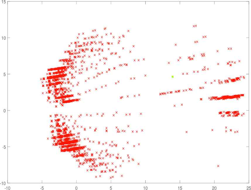
The solution distribution of INS-30-1 with traveling time function 1.
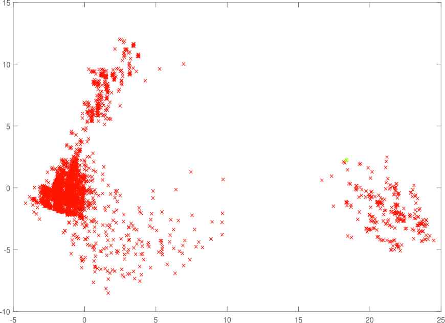
The solution distribution of INS-30-1 with traveling time function 2.
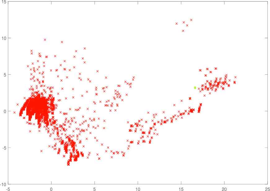
The solution distribution of INS-30-1 with traveling time function 3.
4. DISCUSSIONS
For NP-hard problems, there are three popular approaches to solve the problem, namely, 1) exact algorithms, 2) approximation algorithms, 3) heuristic (or metaheuristic) algorithms. Firstly, the exact algorithms guarantee to find the optimal solution and take exponential time in the worst case, but they often run much faster in practice. The best exact algorithms solve the TDTSP with the instances with up to 50 vertices [6,24,36]. Secondly, an α-approximation algorithm produces a solution within some factor of α of the optimal solution. However, the best approximation ratio is often far from the optimal solution. Thirdly, metaheuristic algorithms perform well in practice and validate their empirical performance on an experimental benchmark of interesting instances. The TDTSP-PD is NP-hard; therefore the metaheuristic algorithm is a natural approach to solve large instances in a short time.
Generally speaking, metaheuristic algorithms can get stuck into local optimum because there is a lack of the balance between diversification and intensification in which diversification means generating diverse solutions to explore the search space on a global scale. In contrast, intensification means to focus on the search in a local region by exploiting the information that a current good solution is found in this region. While the algorithms in [3,4,28] might have a strong search intensification, their diversification mechanisms may not be sufficient. Due to the random nature, population-based algorithms improve on the chance of finding a globally. The same idea can be found in [39–41].
To the best of our knowledge, a population-based algorithm has never been proposed for the TDTSP-PD in the literature. To tackle this computationally challenging problem, we present the first MA for the TDTSP-PD. The MA [29] is a robust population-based framework that combines the exploration from the GA and LS optimization's exploitation capacity. This work's main contributions can be summarized as follows: 1) from the algorithmic perspective, the proposed MA that brings the advantages of the GA and LS maintains the balance between diversification and intensification. In our algorithm, the GA is used to explore the promising solution areas that are yet refined while the VNS exploits them with the hope of improving a solution; 2) from the computational perspective, our algorithm obtains good solutions fast. Compared with the TS+VNS algorithm [28] in 900 instances, the proposed algorithm reaches better solutions in 407 cases and the same solutions in 203 cases. We also adapt the proposed algorithm for the TDTSP case. Our algorithm shows the proposed algorithm's highly competitive performance compared to the state-of-the-art algorithms for the TDTSP [3,28]. Moreover, the proposed algorithm finds the new best solutions in 69 out of 120 cases. It is a significant improvement because the algorithms in [3,28] are the best algorithms in current for the problem. Wilcoxon's test's statistical results also show the clear dominance of the proposed algorithm in comparison with the state-of-the-art algorithms in the literature. A research topic is increasing our algorithm's efficiency and running time to allow even larger problems to be solved in the future.
5. CONCLUSIONS
In this work, the TDTSP in Post Disaster is studied. As our main contribution, we propose a MA that combines the GA and LS to solve the problem. In our algorithm, the GA is used to explore the promising solution areas that are yet refined, while the VNS exploits them with the hope of improving a solution. The proposed algorithm maintains a balance between intensification and diversification. The performance of the proposed MA is evaluated on benchmark datasets for the TDTSP-PD and TDTSP. For the TDTSP-PD, the proposed algorithm finds high-quality solutions when the average gap from the UB is from 14.05% to 18.10%. Compared with the algorithm [28], the proposed algorithm obtains better solutions in 407 and the same results in 203 out of 900 cases. For the TDTSP, our algorithm can find the new best-known solutions for 69 TDTSP-instances. In addition, the instances with 100 vertices can be solved exactly in a short time. Wilcoxon's test's statistical results also show the clear dominance of the proposed algorithm in comparison with the state-of-the-art algorithms in the literature. A research topic is increasing our algorithm's efficiency and running time to allow even larger problems to be solved in the future.
CONFLICT OF INTEREST
The author declares there is no Conflict of Interest.
AUTHORS' CONTRIBUTION
The author designed and implemented the algorithms.
ACKNOWLEDGMENTS
This research is funded by Hanoi University of Science and Technology (HUST) under grant number T2020-PC-008.
APPENDIX
 |
LES, levels of earthquake severity; MA, Memetic Algorithm; TDTSP-PD, Time-Dependent Traveling Salesman Problem in Postdisaster; TS, Tabu Search; UB, upper bound; VNS, Variable Neighborhood Search.
 |
LES, levels of earthquake severity; MA, Memetic Algorithm; TDTSP-PD, Time-Dependent Traveling Salesman Problem in Postdisaster; TS, Tabu Search; UB, upper bound; VNS, Variable Neighborhood Search.
The experimental results for TDTSP-PD with INST-30-x instances that are proposed by [25] (LES = 2).
 |
LES, levels of earthquake severity; MA, Memetic Algorithm; TDTSP-PD, Time-Dependent Traveling Salesman Problem in Postdisaster; TS, Tabu Search; UB, upper bound; VNS, Variable Neighborhood Search.
The experimental results for TDTSP-PD with INST-30-x instances that are proposed by [25] (LES = 3).
 |
LES, levels of earthquake severity; MA, Memetic Algorithm; TDTSP-PD, Time-Dependent Traveling Salesman Problem in Postdisaster; TS, Tabu Search; UB, upper bound; VNS, Variable Neighborhood Search.
The experimental results for TDTSP-PD with INST-30-x instances that are proposed by [25] (LES = 4).
 |
LES, levels of earthquake severity; MA, Memetic Algorithm; TDTSP-PD, Time-Dependent Traveling Salesman Problem in Postdisaster; TS, Tabu Search; UB, upper bound; VNS, Variable Neighborhood
The experimental results for TDTSP-PD with INST-30-x instances that are proposed by [25] (LES = 5).
 |
LES, levels of earthquake severity; MA, Memetic Algorithm; TDTSP-PD, Time-Dependent Traveling Salesman Problem in Postdisaster; TS, Tabu Search; UB, upper bound; VNS, Variable Neighborhood
The experimental results for TDTSP-PD with INST-50-x instances that are proposed by [25] (LES = 1).
 |
LES, levels of earthquake severity; MA, Memetic Algorithm; TDTSP-PD, Time-Dependent Traveling Salesman Problem in Postdisaster; TS, Tabu Search; UB, upper bound; VNS, Variable Neighborhood Search.
The experimental results for TDTSP-PD with INST-50-x instances that are proposed by [25] (LES = 2).
 |
LES, levels of earthquake severity; MA, Memetic Algorithm; TDTSP-PD, Time-Dependent Traveling Salesman Problem in Postdisaster; TS, Tabu Search; UB, upper bound; VNS, Variable Neighborhood Search.
The experimental results for TDTSP-PD with INST-50-x instances that are proposed by [25] (LES = 3).
 |
LES, levels of earthquake severity; MA, Memetic Algorithm; TDTSP-PD, Time-Dependent Traveling Salesman Problem in Postdisaster; TS, Tabu Search; UB, upper bound; VNS, Variable Neighborhood Search.
The experimental results for TDTSP-PD with INST-50-x instances that are proposed by [25] (LES = 4).
 |
LES, levels of earthquake severity; MA, Memetic Algorithm; TDTSP-PD, Time-Dependent Traveling Salesman Problem in Postdisaster; TS, Tabu Search; UB, upper bound; VNS, Variable Neighborhood Search.
The experimental results for TDTSP-PD with INST-50-x instances that are proposed by [25] (LES = 5).
 |
LES, levels of earthquake severity; MA, Memetic Algorithm; TDTSP-PD, Time-Dependent Traveling Salesman Problem in Postdisaster; TS, Tabu Search; UB, upper bound; VNS, Variable Neighborhood Search.
The experimental results for TDTSP-PD with INST-100-x instances that are proposed by [25] (LES = 1).
 |
LES, levels of earthquake severity; MA, Memetic Algorithm; TDTSP-PD, Time-Dependent Traveling Salesman Problem in Postdisaster; TS, Tabu Search; UB, upper bound; VNS, Variable Neighborhood Search.
The experimental results for TDTSP-PD with INST-100-x instances that are proposed by [25] (LES = 2).
 |
LES, levels of earthquake severity; MA, Memetic Algorithm; TDTSP-PD, Time-Dependent Traveling Salesman Problem in Postdisaster; TS, Tabu Search; UB, upper bound; VNS, Variable Neighborhood Search.
The experimental results for TDTSP-PD with INST-100-x instances that are proposed by [25] (LES = 3).
 |
LES, levels of earthquake severity; MA, Memetic Algorithm; TDTSP-PD, Time-Dependent Traveling Salesman Problem in Postdisaster; TS, Tabu Search; UB, upper bound; VNS, Variable Neighborhood Search.
The experimental results for TDTSP-PD with INST-100-x instances that are proposed by [25] (LES = 4).
 |
LES, levels of earthquake severity; MA, Memetic Algorithm; TDTSP-PD, Time-Dependent Traveling Salesman Problem in Postdisaster; TS, Tabu Search; UB, upper bound; VNS, Variable Neighborhood Search.
The experimental results for TDTSP-PD with INST-100-x instances that are proposed by [25] (LES = 5).
REFERENCES
Cite this article
TY  - JOUR
AU  - Ha-Bang Ban
PY  - 2021
DA  - 2021/03/17
TI  - Applying Metaheuristic for Time-Dependent Traveling Salesman Problem in Postdisaster
JO  - International Journal of Computational Intelligence Systems
SP  - 1087
EP  - 1107
VL  - 14
IS  - 1
SN  - 1875-6883
UR  - https://doi.org/10.2991/ijcis.d.210226.001
DO  - 10.2991/ijcis.d.210226.001
ID  - Ban2021
ER  -