
Fuzzy Hoeffding Decision Tree for Data Stream Classification
 , Francesco Marcelloni1, , Riccardo Pecori2, *,
 - DOI
- 10.2991/ijcis.d.210212.001How to use a DOI?
- Keywords
- Streaming data classification; Fuzzy decision tree; Hoeffding decision tree; Model interpretability
- Abstract
Data stream mining has recently grown in popularity, thanks to an increasing number of applications which need continuous and fast analysis of streaming data. Such data are generally produced in application domains that require immediate reactions with strict temporal constraints. These particular characteristics make problematic the use of classical machine learning algorithms for mining knowledge from these fast data streams and call for appropriate techniques. In this paper, based on the well-known Hoeffding Decision Tree (HDT) for streaming data classification, we introduce FHDT, a fuzzy HDT that extends HDT with fuzziness, thus making HDT more robust to noisy and vague data. We tested FHDT on three synthetic datasets, usually adopted for analyzing concept drifts in data stream classification, and two real-world datasets, already exploited in some recent researches on fuzzy systems for streaming data. We show that FHDT outperforms HDT, especially in presence of concept drift. Furthermore, FHDT is characterized by a high level of interpretability, thanks to the linguistic rules that can be extracted from it.
- Copyright
- © 2021 The Authors. Published by Atlantis Press B.V.
- Open Access
- This is an open access article distributed under the CC BY-NC 4.0 license (http://creativecommons.org/licenses/by-nc/4.0/).
1. INTRODUCTION
During the last years, the analysis of data streams is getting more and more attention because of the huge number of different sources of streaming data we get in touch everyday. These can be simple sensors, but also wearables, smartphones, as well as all other smart devices of the Internet of Things environment [1]. Other examples of data stream sources may entail tools for the continuous measurement and monitoring of network traffic [2], web surfing logs [3], networked manufacturing machines in Industry 4.0 [4,5], virtual learning environments [6], online social networks [7], etc.
In the context of data streams, data are usually collected at very high rates, imposing strict temporal constraints and important challenges to the algorithms used for machine learning and data mining. These challenges can be briefly summarized as follows:
the practical availability of limited resources compared to the theoretically infinite quantity of data in a stream. Indeed, machine learning algorithms should consider an instance only once and get immediate information for training the models, limiting as much as possible the amount of stored data;
the changes over time of the distribution of the data, a phenomenon also known as concept drift which should be properly faced and addressed;
the necessity for the models, which are continuously updated as data arrive, to make accurate predictions at any time [8].
As a consequence, following the aforementioned three challenges, three corresponding metrics, mutually dependent, are usually considered in the design of models for data streams. They are the following: accuracy in the predictions, quantity of memory to store training data, and time needed for learning the model itself [9]. The concurrent optimization of the aforementioned three metrics, which should take place in the initial learning phase, is a very difficult and demanding task, just because of the already mentioned mutual dependence: improving accuracy generally requires more memory and time, and vice versa.
In this paper, we describe a new approach for the incremental learning of multi-way Fuzzy Decision Trees (FDTs), which has been preliminaryly introduced in Ref. [10]. In particular, we take advantage of the main characteristics of the traditional Hoeffding Decision Tree (HDT) [11], a decision tree purposely proposed for managing data stream classification, and extend it with fuzziness by adopting some of the concepts of the FDT proposed by Segatori et al. [12]. In particular, we choose the best input attribute to be used for the splitting at each decision node, by means of the fuzzy information gain (FIG) proposed in Ref. [12]. Unlike Ref. [12], for the sake of simplicity, we adopt for each input attribute, fuzzy uniform partitions.
We have tested the proposed incremental learning procedure for building FDTs on five datasets for data stream classification. Specifically, we adopted three synthetic datasets on which researchers usually carry out experiments for the analysis of concept drifts in streaming data [13–16]. Moreover, we selected two datasets which are related to real-world applications, namely the optical recognition of handwritten digits and the detection of the presence or absence of people in a room. As regards the latter, it is a typical Smart Building application [17,18], suitable for taking the decision of switching off power consuming devices, whenever the room is empty.
An extensive experimental analysis has been carried out, considering different strategies for simulating the data streaming and for analyzing the generated models in terms of their classification performance and model complexity and interpretability. We have compared the proposed FDT, denoted as Fuzzy HDT (FHDT) in the following, with the traditional HDT. Moreover, as regards the room occupancy dataset, we have also compared the results achieved by both FHDT and HDT with the ones presented in the paper where the dataset has been introduced [18] and with ones achieved by a recent fuzzy clustering-based algorithm for data streaming classification [19].
The experiments show that FHDT achieves very good results in terms of classification, performance, and complexity, especially for the dataset characterized by the presence of concept drifts, such as the synthetic datasets and the occupancy dataset. Moreover, the exploitation of uniform fuzzy partitions allows us to extract, from FHDT, simple, accurate, and explainable fuzzy rules.
Compared to Ref. [10], we have added the following further contributions:
we have tested the novel FHDT considering three synthetic datasets and an additional real-world application, namely the room occupancy detection;
we have compared FHDT and HDT experimenting different data splitting scenarios for simulating the data streaming;
as regards the two real-world datasets, we have evaluated both FHDT and HDT considering two modalities, namely the classical test-the-train strategy and using pre-defined test sets.
The rest of the paper has the following structure. Section 2 summarizes some recent work about data stream mining, with particular emphasis on decision trees and FDTs. In Section 3, we report some background about fuzzy partitioning and the structure of an FDT. In Section 4, we delve into the proposed incremental procedure for learning FHDTs, describing it in detail. In Section 5, we present the results of the experimental campaign carried out on the considered datasets. Section 6 draws some conclusions and discusses some future work.
2. RELATED WORK
HDT [11], also known as “Very Fast Decision Tree”, is a reference model to classify streaming data. HDT encompasses a learning strategy to create a decision tree in an incremental way, storing in memory only the necessary statistics. In particular, the growing of the tree entails the splitting of one leaf whenever it contains a minimum number of instances and a condition based on the Hoeffding's theorem is met. In particular, the theorem defines a bound which decreases with the increase of the number of instances. The condition is verified when the difference between the two highest values of the information gains computed for the attributes available at the decision node is higher than the bound. In Ref. [11], the authors state that this bound guarantees, with a given level of confidence, that the attribute chosen for the splitting is the same as the one that would have been selected after analyzing the infinite sequence of instances. The theoretical justification based on the Hoeffding's theorem has been criticized in some papers published in the last years [20–22]. The authors of these papers contest the applicability of the Hoeffding's theorem to the information gain. Ref. [21] claims that “the bound obtained in Ref. [11] cannot be justified using Hoeffding's theorem. However, it still can be considered as a heuristic method, which gives satisfactory practical results.” Actually, HDT has been implemented in some software packages and is commonly used in streaming data classification.
During the last years, some solutions to improve the HDT learning have been proposed. For example, the authors of Ref. [23] have proposed an approach to address the concept drift issue. Moreover, the contribution in Ref. [24] has introduced a method to deal with noisy instances as well as to manage the dimension of the tree. In Ref. [25], Kourtellis et al. have presented Vertical HDT, a parallel and distributed version of the incremental HDT learning procedure, which has been successfully tested on big streaming data.
Regarding fuzzy logic and fuzzy set theory, they have been recently used in decision tree models, both considering batch and streaming scenarios. As a matter of fact, when fuzzy sets are employed to discretize the domains of the attributes used in these classifiers, vague and noisy data can be handled in a very efficient way [26–29]. An introduction on theoretical issues and methods on FDTs can be found in Ref. [30]. The work of Umanol et al. [31] represents one of the first contributions on FDTs: the authors discuss the application of a fuzzy version of the well-known ID3 algorithm for diagnosis systems. The contribution of Segatori et al. [12] presents a recent technique to train binary and multi-way FDTs in batch mode for big data classification. In particular, the authors take advantage of a fuzzy partitioning of the input attributes, performed through a novel distributed discretizer, and employ the FIG to choose the splitting attributes in the decision nodes of the tree. More recently, Barsacchi et al. [32] have introduced a method for building ensembles of binary FDTs based on an AdaBoost-like boosting method.
As regards streaming data classification, the work discussed in Ref. [26] introduces one of the first approaches for incremental learning of an FDT. The proposed learning algorithm is based on the main scheme discussed in Ref. [11], but it is improved by introducing a new technique called Threaded Binary Search Tree, which allows a more efficient control of the candidate splitting points. In order to improve noisy data handling, a soft discretization is adopted along with a fuzzy version of the information gain. The Flexible FDT (FlexDT) [27] is another example of FDT proposed in the literature to handle the classification of streaming data. FlexDT is grounded on the same incremental learning procedure of the traditional HDT, but it exploits binary fuzzy partitions for each attribute at the internal decision nodes. The authors have employed sigmoidal fuzzy sets and defined proper heuristics in order to tune their parameters in the learning stage. The Hoeffding bound and the information gain, in their traditional definitions, are used in order to, respectively, decide if growing or not the tree and choose the best possible attribute for the splitting at each decision node.
An extension of FlexDT, Multi FlexDT, has been introduced in Ref. [28]. Multi FlexDT employs multi-way rather than binary splits at each internal decision node. When a new decision node is created, a binary fuzzy partition is adopted as in FlexDT, but, subsequently, the incremental learning algorithm creates a new binary partition for the attribute at the arrival of a new training instance whose membership degree to each fuzzy set is lower than a certain threshold. In this way, the previous partition is extended at each decision node by taking the two new sigmoidal fuzzy sets into account, thus considering the two new splittings. A further extension of Multi FlexDT, called MHFlexDT, has been recently discussed in Ref. [29]. Here, the authors have proposed to use the McDiarmid bound rather than the Hoeffding bound for checking the splitting conditions at the decision node. In the experiments, MHFlexDT has proved to better control the depth of the tree than Multi FlexDT.
Two common characteristics of FlexDT, Multi FlexDT, and MHFlexDT are: i) the incremental generation of noise-robust models and ii) the efficient management of missing values. Nevertheless, some drawbacks regard the impossibility of i) defining a-priori linguistic labels for each input attribute and ii) ensuring a good level of integrity for the fuzzy partitions. Therefore, the interpretability of the aforementioned FDTs may not be always guaranteed.
In the specialized literature, also different fuzzy models can be found for mining useful knowledge from data streams in real-time. These models belong to the “Evolving Fuzzy Systems” [33] research branch, which includes fuzzy rule-based systems, fuzzy pattern trees (FPTs), semi-supervised approaches based on fuzzy clustering, and, obviously, FDTs. A recent survey on Evolving Fuzzy Systems has been published by Škrjanc et al. [34] in 2019.
In 2004, Plamen and Filev published one of the pioneer work in the framework of Evolving Fuzzy Systems [35], in which they discussed an incremental approach for learning Takagi–Sugeno fuzzy rule-based systems. Along the years, several extensions and applications to different fields have interested evolving fuzzy rule-based systems [36,37].
In 2013, Shaker et al. [14] discussed an evolving version of the so called FPTs for binary classification. An FPT is a tree-like structure different from classical decision trees. Indeed, its inner nodes represent fuzzy operators whereas leaf nodes are associated with fuzzy predicates employing input attributes. The input of a pattern tree is entered at the leaf nodes and its membership degree to each leaf is calculated and propagated to the parent nodes until reaching the root where a real value in [0,1] is generated. Using a threshold function, the input is classified in one of the two classes.
Finally, Casalino et al. recently introduced the Dynamic Incremental Semi-Supervised FCM (DISSFCM) classification algorithm [19,38]. DISSFCM is based on an extended version of the well-known fuzzy C-means algorithm and has been designed for handling streaming data, even in a semi-supervised fashion. The incremental learning algorithm is capable to dynamically adapt the number of clusters to data streams.
3. THEORETICAL BACKGROUND
In this section, we introduce the theoretical background our work is grounded on. It mainly concerns the theory about fuzzy partitions, the structure of an FDT as well as of a traditional HDT.
3.1. Fuzzy Partitions
Let
In this work, we adopt strong and uniform triangular fuzzy partitions [39]. Figure 1 shows an example of these partitions made up of three triangular fuzzy sets Af,j, whose membership function is represented by the tuples (af,j, bf,j, cf,j), where af,j and cf,j correspond to the left and right extremes of the support of Af,j, and bf,j to its core.
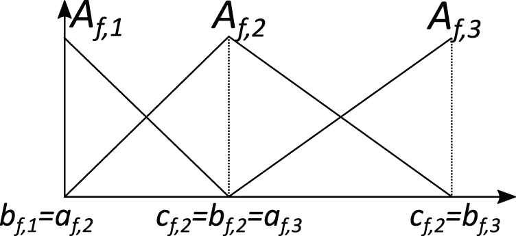
Example of a strong fuzzy partition with three triangular fuzzy sets.
3.2. Fuzzy Decision Trees
A decision tree can be defined as a directed acyclic graph, wherein internal nodes perform a test on an attribute, branches represent the outcome of the test, and terminal nodes, i.e., leaves, contain instances belonging to one or more class labels. The first node to be created is named “root” of the tree. Generally, in each leaf node, class Γk ∈ Γ is associated with a weight wk determining the strength of class Γk in the leaf node itself.
Let
First of all, one of the attributes is chosen at the root, taking into consideration the overall TR, and a set of branches and corresponding nodes is returned. A branch corresponds to a condition on the values of the attribute. For each node, a new attribute is selected from the set of the attributes, considering only the instances of TR satisfying the test associated with the branch. When no attribute can be selected, the node is considered as a leaf. The attribute selection is based on a metric, which is usually either the Information Gain or the Gini Index [40].
In this paper, we adopt a multi-way FDT exploiting FIG [12] as attribute selection metric. First of all, each attribute is partitioned. For the sake of simplicity, we set the same value of Tf = Tmax for each attribute. In multi-way FDTs, each test node has exactly a number of branches equal to the number of fuzzy sets in the partition of the attribute selected in the node. Thus, in our case, each test node has Tmax branches. Figure 2 shows an example of multi-way FDT, where we represent only two attributes: X2 at the root and X1 at the second level. All attributes are partitioned into three fuzzy sets, thus generating exactly three output branches. In the example, for the sake of simplicity, each leaf is associated with just one class.
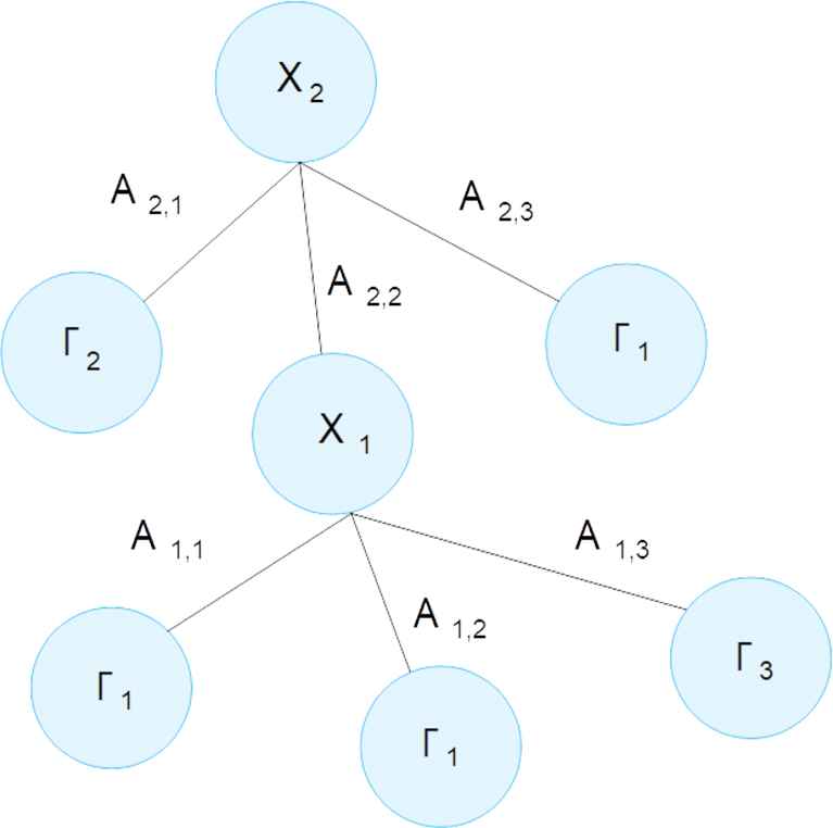
Example of multi-way FDT with only two levels and one single class per leaf.
In the learning phase, the root contains the whole TR and each FDT node contains the subset of instances in TR which has a membership degree different from 0 to the node. The FDT construction starts from the root and follows a top-down approach; unless a termination condition is satisfied, a node gives rise to Tmax child nodes according to the fuzzy partition of the attribute chosen for the splitting. The chosen attribute is the one that yields the highest FIG, which will be defined below.
More formally, given a parent node P, let Cj indicate the generic jth child node, j = 1, …, Tmax. The subset of TR in Cj contains only the instances belonging to the support of the fuzzy set Af,j. Let SP be the set of instances in the parent node, and
The FIG used for selecting the splitting attribute is computed, for a generic attribute Xf with partition Zf, as
Once the learning phase has terminated and the tree has been built, a given unlabeled instance
Finally, the output class of the unlabeled instance
maximum matching: the output class is the one corresponding to the maximum association degree computed for the instance;
weighted vote: the output class is the one corresponding to the maximum total strength of vote, computed by summing all the activation degrees in each leaf for the class.
In this work, we have employed the weighted vote approach.
3.3. The Incremental Learning Procedure of HDT
In this subsection, we briefly summarize the iterative learning procedure of the traditional HDT. Whenever a new label instance of the stream is processed, the HDT learning procedure updates the current structure of the decision tree by means of two main steps: i) refresh of the class statistics in the nodes and leaves and ii) possible growth of the tree. This procedure depends on the following parameters:
Grace Period (GP): a threshold on the number of instances contained in one leaf before considering it for a split;
Tie Threshold (TT): a threshold to break the ties forcibly if the difference between the information gains of the two attributes with the highest information gains is too small. This avoids waiting for too much time before a splitting event;
Split Confidence (δ): a metric involved in the direct computation of the Hoeffding Bound;
Minimum Fraction (MF): the minimum percentage of instances in a branch after a possible split of a leaf.
Regarding the first step, the procedure starts from the root of the tree, determines the leaf reached by the current instance and updates its per-class statistics as well as the cardinality (total number of crisp instances) of the leaf itself. After that, some checks are performed in order to decide if splitting or not the current leaf L and therefore growing the tree (second step).
First of all, the splitting is not permitted whenever the number of instances, i.e., the Cardinality (NL) in L is lower than GP.
If this check is passed, attributes are ranked according to their Information Gain and the Hoeffding Bound (HBL) at the current leaf L is computed as:
Afterward, the difference between the information gains of the first two attributes in the ranking is computed. If this difference is higher than HBL or HBL is lower than TT, then the splitting of L is permitted and is performed by employing the attribute with the highest information gain as the splitting attribute. Indeed, a final check is performed before the splitting is actually carried out: this check regards the percentage of instances in each post-split branch, which should be greater than MF for the splitting process to be completed.
The creators of HDT claimed in Ref. [11] that the splitting procedure employs the Hoeffding bound to ensure, with high probability, that the attribute chosen for the splitting, by using the subset of instances corresponding to the cardinality at the current leaf, is the same as the one that would be chosen using an infinite number of instances [11]. As we have already highlighted in Section 2, some subsequent papers have contested the applicability of the Hoeffding's theorem to the estimation of the information gains, thus making the Hoeffding bound used in the HDT learning approach a heuristic rather than a theoretically-based threshold. The use of this heuristic in the last years has, however, proved that it ensures satisfactory practical results. In the next section, we adapt the heuristic proposed in Ref. [11] to the fuzzy domain to take into consideration that, considering the fuzzy partitions used in this paper, one instance can belong to different nodes at each tree level (except the root), with different membership degrees.
4. THE PROPOSED STREAM FDT
The incremental learning procedure of FHDT is based on that one employed in the standard HDT, apart from the following two aspects:
the procedure to update the statistics at a particular leaf;
the use of a similar but different metric for selecting the best splitting attribute, i.e., the FIG.
Concerning the first aspect, the learning procedure starts from the root and follows the paths activated by the current training instance until leaves are reached. Unlike the traditional HDT, where an instance can reach only one leaf, in the proposed FHDT a training instance can reach more than one leaf. This happens because an instance triggers more than one branch in a splitting node. Indeed, an instance can belong to different fuzzy sets in a partition of an attribute with different membership degrees. In the scenario we consider in this paper, i.e., strong uniform partitions, only two output branches can be activated simultaneously at each decision node. Once an instance, traveling throughout the tree, reaches a leaf node, the membership degree to the node is calculated according to Eq. (1). Furthermore, the fuzzy cardinality of the leaf node and the fuzzy cardinalities of the leaf node per each class represented in the node are updated exploiting Eq. (2) with, respectively, all the instances belonging to the leaf node and with the subset of these instances labeled with a specific class.
Regarding the second aspect, the learning procedure verifies whether the conditions to allow the growth of the FHDT by splitting one of the current leaves are satisfied. Since each instance belonging to a leaf L with a membership degree higher than 0 may also belong to other children (only one with the uniform partitions used in this paper) of the same parent P, we modified the Hoeffding bound in Eq. (7) to take this aspect into consideration. Indeed, instead of computing the cardinality NL as the sum of the instances belonging to the leaf, we compute it as the sum of the membership degrees of the instances in P to the fuzzy set associated with the branch leading to L. We denote this cardinality as local fuzzy cardinality LFCL of L. Let Af,j be the fuzzy set associated with the branch which links P to L. Formally, LFCL is defined as:
If the LFCL is greater than GP, then the algorithm sorts the attributes Xf according to their FIG computed as in Eq. (3). Therefore, it computes the difference between the FIGs of the first two attributes in the ranking: if the difference is higher than FHBL or FHBL is lower than TT, then L is split. The attribute with the highest FIG is considered as splitting attribute. The splitting is actually performed if
We would like to highlight that in our proposed learning procedure for FHDT, we adopted LFCL rather than NL in the conditions to start the splitting procedure. This decision is intuitively supported by the fact that the uncertainty associated with the arrival of a new instance is spread among the different paths of the FHDT rather than in a single path as in the case of HDT. It should be noticed that, since the maximum value of the fuzzy cardinality of an instance in L is equal to 1, NL can be considered as an upper bound for LFCL. Therefore, FHBL can be regarded as an upper bound for HBL and, thus, the splitting condition used in our FHDT, namely FIG(Xbest)L − FIGL(XnextBest)L > FHBL, is more restrictive than the one checked in the traditional HDT. This allows collecting a higher number of instances and to have a higher confidence on the decision of splitting the leaf.
Algorithm 1 summarizes the FHDT learning algorithm in pseudo-code. In the code, Xϕ represents the null attribute that consists in not splitting the node. For each new training instance, the algorithm checks the conditions for splitting each leaf and, if the conditions are satisfied, replaces the leaf with an internal node and adds a number of new leaves corresponding to the number of possible values for the attribute chosen for the splitting.
Algorithm 1: Algorithm to learn an FHDT.
1: Input: S: the stream of training instances, X: the set of numeric attributes, FIG(.): the fuzzy information gain, δ: one minus the probability of choosing the correct attribute at any given node.
2: Output: one FHDT
3: Let FHDT be a fuzzy decision tree with a single leaf L (root)
4: Let
5: for each training instance in S do
6: for each leaf L do
7: Update statistics of leaf L needed to compute the conditions for deciding the splitting
8: Compute LFCL, the sum of the fuzzy cardinality over all classes at leaf L
9: if LFCL > GP then
10: for each attribute
11: Compute
12: Let Xa be the attribute with the highest
13: Let Xb be the attribute with the second-highest
14: fuzzy Hoeffding Bound FHBL
15: if
16: Replace L with an internal node splitting on
17: Add a new leaf
18: end if
19: end if
20: end for
21: end for
5. SIMULATIONS AND RESULTS
In this section, first of all we describe the synthetic and real-world datasets and the simulation scenario in which they were experimented. Then, we present and discuss the results achieved by the proposed FHDT and compare them to the ones obtained by HDT. Specifically, we first describe the analysis carried out on synthetic datasets and then the analysis carried out on real-world datasets.
5.1. Datasets
We evaluate the effectiveness of the proposed FHDT by considering two categories of datasets, namely synthetic and real-world datasets, simulating their evolution over time.
As regards synthetic datasets, we adopted the SEA concepts and Rotating Hyperplane datasets, which have been extensively used in several contributions on data stream classification, especially for the analysis of the concept drift [13–16].
The SEA concepts dataset (SEA dataset, in short) regards data characterized by an abrupt concept drift. It considers three input attributes whose values are randomly generated in the range [0,10) and only the first two attributes are relevant. An instance belongs to the positive class if the sum of the first two attribute values is lower than a threshold θ, otherwise it belongs to the negative class. Different values of θ are usually adopted in order to generate different concepts. We adopted a version of the dataset, available on a web repository,a composed of 50,000 instances with four different concept drifts.
The Rotating Hyperplane dataset regards data characterized by a gradual concept drift. It is generated from a d-dimensional hyperplane described by the equation
Details on the parameters and the procedures for generating the three synthetic datasets, namely SEA, Hyperplane5, and Hyperplane9, can be found in Ref. [13].
As regards real-world datasets, they have been extracted from the UCI machine learning repository and are:
the Optical Recognition of Handwritten Digits dataset (Handwritten digits dataset, in short)b;
the Occupancy Detection dataset (Occupancy dataset, in short).c
The first real-world dataset contains normalized bitmaps of handwritten digits which represent 10 different classes (digits ranging from zero to nine). This dataset comes from 32 × 32 bitmaps, divided into 4 × 4 nonoverlapping blocks, wherein the number of pixels are counted. This subdivision generates an input matrix of 8 × 8, where each element is an integer in the set [0…16]. Therefore, each image represents an instance characterized by 64 numerical attributes with integer values [0…16], and one class attribute in [0…9]. A total of 5,620 samples are included in the dataset and, similarly to the experimental scenario adopted in Ref. [38], we considered 10% of them as a test set and the remainder as a training set. Both training and test sets maintain the original uniform class distribution. Table 1 summarizes the characteristics of the Handwritten digits dataset.
| Dataset | Instances | Single Class Distribution |
|---|---|---|
| Training set | 5,058 | 10% |
| Test set | 562 | 10% |
| Full dataset | 5,620 | 10% |
Characteristics of the Handwritten digits dataset.
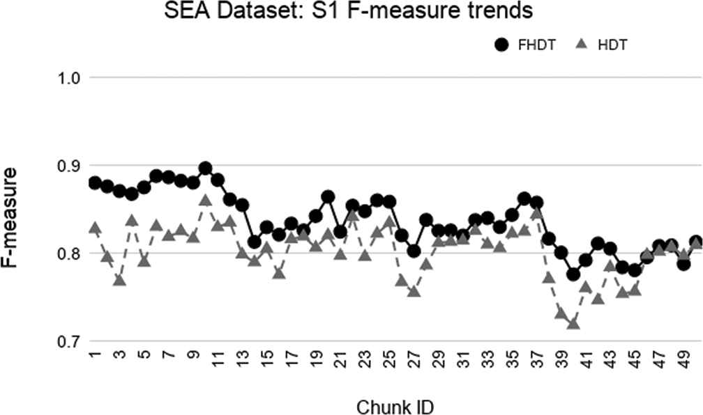
Test-the-train experiment: weighted F-measure trends for S1 on the SEA dataset.
The second real-world dataset concerns the occupancy detection in a room, namely a binary classification task about the presence or absence of people. This dataset regards a real application in the framework of Smart Buildings [17]. Indeed, the information on the occupancy of a room can be used in order to switch off lights, ventilation, and all the energy-based equipment to save energy and enact possible safety actions. This dataset was introduced in Ref. [18] and recently adopted in the experiments carried out in Ref. [19]. In this dataset, each data sample encompasses five attributes: Temperature (Celsius), Relative Humidity (%), Light (Lux), CO2 (ppm), Humidity Ratio (kg of water-vapor per kg of air), which have been measured every minute in a room in the period from Feb. 3, 2015 to Feb. 10, 2015. Each sample belongs to one out of two possible classes, namely “non-occupied room” and “occupied room”. Therefore, the dataset is structured as a stream of 20 560 chronologically sorted data samples, divided into a training set and two test sets, which differ in the room conditions. In the first test set, similarly to the training set, the measurements have been taken mostly with the door closed during the occupied status, while in the second test set the measurements have been taken mostly with the door open during the occupied status. Table 2 reports some basic statistics on the data and on the class distribution of the Occupancy dataset.
| Dataset | Instances | Class Distribution |
|
|---|---|---|---|
| Non Occupied Room | Occupied Room | ||
| Training | 8,143 | 79% | 21% |
| Test 1 | 2,665 | 64% | 36% |
| Test 2 | 9,752 | 79% | 21% |
Characteristics of the Occupancy dataset.
In the experiments, we have normalized, for all the datasets, the values of each attribute to vary in the interval [0, 1], thus the universe Uf of each attribute Xf ranges from zero to one.
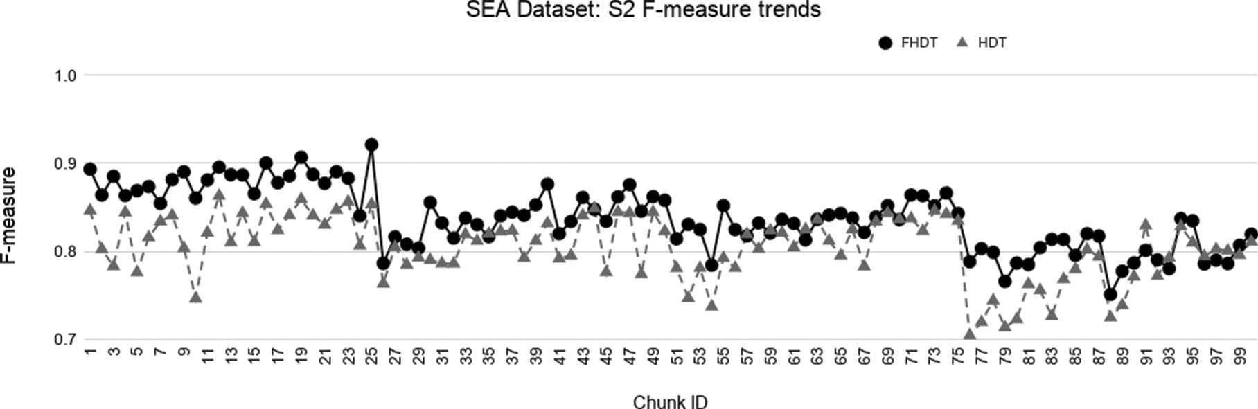
Test-the-train experiment: weighted F-measure trends for S2 on the SEA dataset.
5.2. Simulation Settings
We executed the simulations on a computer featuring an
For all the datasets, the data stream has been simulated by dividing the training sets into a number Q of chunks and then by analyzing the chunks as they arrived in sequence.
For the real-world datasets, similar to the work discussed in Refs. [19,38], we performed two different experiments for both datasets:
Test-the-train: we considered only the training set, opportunely divided into Q chunks. We simulated the data stream by evaluating the performance on the data chunk at the current time interval Tq, with q = 2, … Q, of the current classification model, trained considering the stream of instances included into the data chunks arrived until the time interval Tq−1. During the first time interval T1, the classification model is just built using the first chunk of the dataset.
Test-the-test: the generalization capability of each model incrementally built at the current time interval Tq has been evaluated considering the available test sets. We recall that, as discussed in the previous section, for the Occupancy dataset we have two test sets.
For the real-world datasets, we adopted the same experimental scenarios as those adopted in Refs. [19,38], in which, the authors considered Q equal to 5, 10, 15, and 20 for the Handwritten digits dataset and Q equal to 7, 12, and 17 for the Occupancy dataset, respectively. We labeled this organization of the datasets into different numbers of chunks as S1, S2, S3, and S4, and S1, S2, and S3 for the first and the second real-world dataset, respectively.
For the synthetic datasets, similar to the works discussed in Refs. [13–15], we carried out only test-the-train experiments. Similar to the work in Ref. [13], we adopted experimental scenarios setting Q to 50 and 100 for the SEA dataset, and to 20 and 40 for the Hyperplane5 and Hyperplane9 datasets. Also for the synthetic datasets, we labeled this organization of the datasets into two different numbers of chunks as S1 and S2.
The optimal performance of a classifier for streaming data depends on a fixed set of critical parameters, whose values are conditioned by the particular considered dataset [41]. Thus, we have accomplished a preliminary simulation campaign in order to select the best possible values for the main parameters of both HDT and FHDT, considering the five selected datasets. Table 3 reports these values for both the algorithms: these values have been obtained by searching for an optimal trade-off between increasing the accuracy and reducing the tree depth.
| Parameter | Value |
|---|---|
| Split confidence (δ) | 10−7 |
| Tie threshold (TT) | 2.5 |
| Grace period (GP) | 25 |
| Minimum fraction (MF) | 0.01 |
Values of the main parameters for both HDT and FHDT.
For a fair comparison, we considered the same values of the aforementioned parameters for both the proposed FHDT and the traditional HDT. As regards FHDT, we adopted for each attribute a uniform fuzzy partition consisting of 3 triangular fuzzy sets. Actually, we experimented different configurations considering also 5, 7, and 9 fuzzy sets for partitioning each attribute. The best results, in terms of trade-off between classification performance and complexity (number of nodes and leaves) of the model, have been achieved with 3 fuzzy sets. Thus, for the sake of brevity and readability of graphs and tables, we skipped to show the other results.
5.3. Experimental Results on Synthetic Datasets
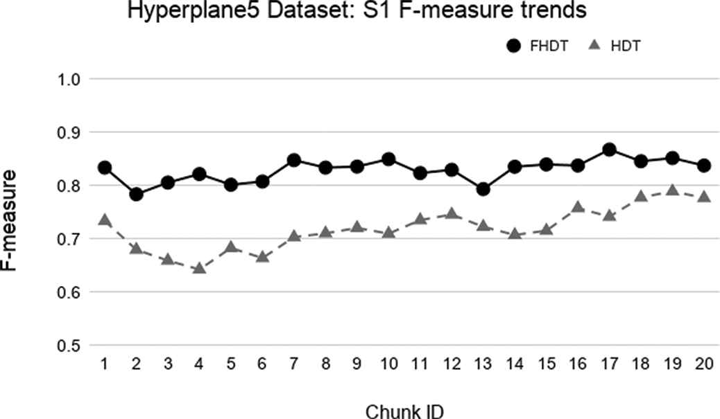
Test-the-train experiment: weighted F-measure trends for S1 on the Hyperplane5 dataset.
In the synthetic datasets, due to the simulated concept drift, the class distribution in the different chunks changes dynamically. For this reason, we adopted the weighed F-measures for evaluating the performance of the classifiers on these datasets. Figures 3–8 show the trends of the weighted F-measures obtained by FHDT and HDT on, respectively, SEA, Hyperplane5, and Hyperplane9, along the sequence of chunks, considering both S1 and S2 chunking strategies. As expected, the concept drift is very accentuated for the SEA datasets. However, it is worth noticing that, both for S1 and S2, FHDT can control this phenomenon better than HDT. Futhermore, in most of the cases, the values of the weighted F-measure achieved by FHDT are higher than the ones achieved by HDT. As regards the two versions of the Hyperplane dataset, the figures show that FHDT outperforms HDT at each chunk of the data stream. It is worth noticing that for Hyperplane9 the concept drift is more evident than for Hyperplane5. Indeed, FHDT controls better the concept variations in the first part of the sequence of chunks, rather than in the last part in which the F-measure drops below 0.8.
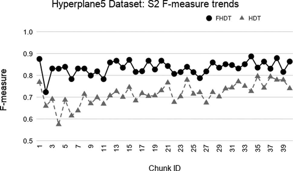
Test-the-train experiment: weighted F-measure trends for S2 on the Hyperplane5 dataset.
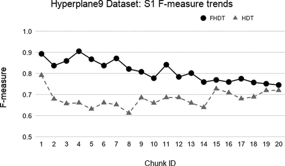
Test-the-train experiment: weighted F-measure trends for S1 on the Hyperplane9 dataset.
As regards the complexity of the generated models, Figures 9–14 show the trends of the total number of nodes of each tree obtained by FHDT and HDT on SEA, Hyperplane5, and Hyperplane9, respectively, along the sequence of chunks, considering both S1 and S2 chunking strategies. For each considered experiment on each dataset, the size of the trees generated by HDT increases linearly while new chunks are fed into the incremental learning algorithm, whereas the sizes of the trees generated by FHDT grow very slowly. Specifically, as regards the SEA dataset, the structure of the trees generated by the FHDT learning algorithm remains stable along the entire flow of data chunks. This is mainly due to the fact that a simple fuzzy tree with 7 nodes and 5 leaves is able to model the instances of the SEA dataset represented in a three-dimensional space. As regards the two Hyperplane datasets, we observe that the FHDTs maintain a stable structure more or less after analyzing the half of the chunks (check Tables 5 and 6 in which this behavior is more evident than in the Figures).
Tables 4–6 show an excerpt of the results, in terms of classification performance and of complexity of the models, for SEA, Hyperplane5, and Hyperplane9 datasets, respectively. In particular, we present the results for the chunks which are characterized by the most evident concept drift. The tables confirm that the FHDTs outperform, in most of the cases, the HDTs in terms of weighted F-measure, thus pointing out a good capability of managing the concept drift. Moreover, the FHDTs are characterized by a much lower complexity level, in terms of their depth, number of nodes, and number of leaves, than the HDTs. This characteristic, along with the use of linguistic terms in the partitions, ensures a much higher level of interpretability of the FHDTs than the HDTs.
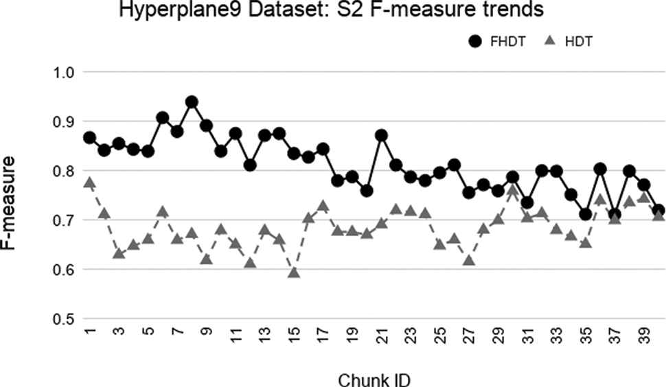
Test-the-train experiment: weighted F-measure trends for S2 on the Hyperplane9 dataset.
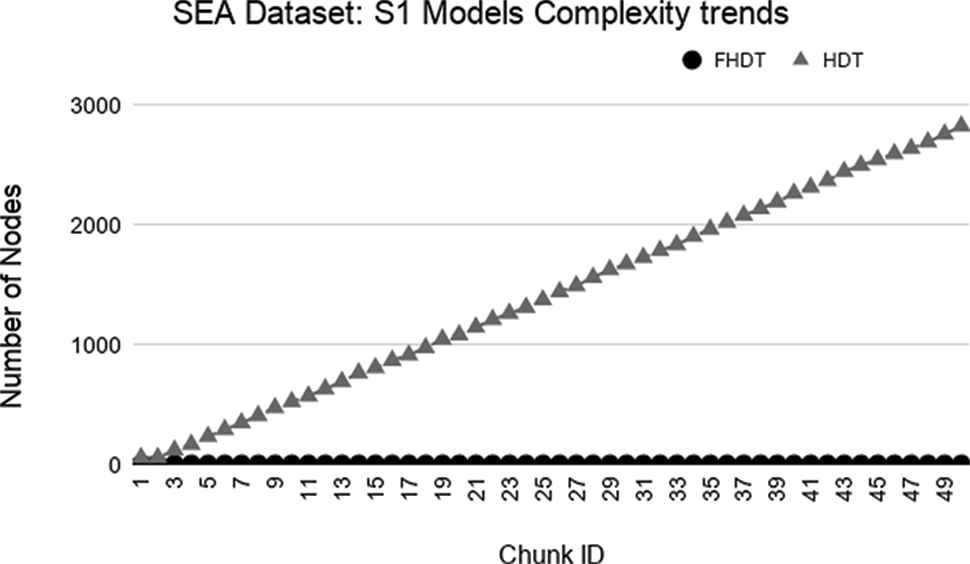
Model complexity trends for S1 on the SEA dataset.
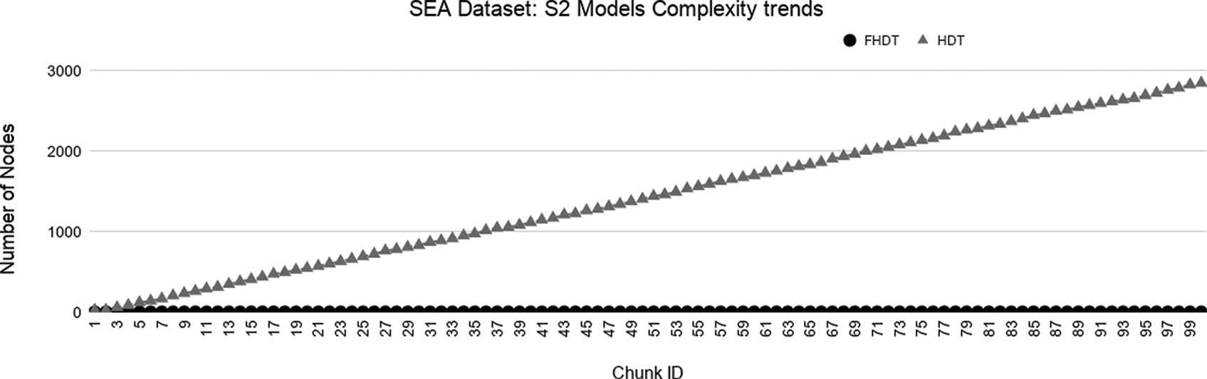
Model complexity trends for S2 on the SEA dataset.
5.4. Experimental Results on Real-World Datasets
5.4.1. Handwritten digits dataset
Figures 15–18 show the trends of the accuracy obtained by FHDT and HDT on S1, S2, S3, and S4, respectively, along the sequence of chunks of the Handwritten Digits dataset (shortened to Handwritten dataset in the following). It is worth noticing that for the first chunk we show the accuracy calculated considering it as training and test set. For the remaining chunks, we show the accuracy calculated considering each chunk q as test set, after an incremental learning process which includes training samples till chunk q − 1.
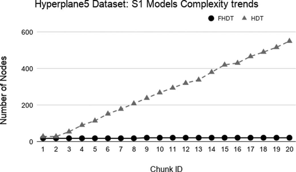
Model complexity trends for S1 on the Hyperplane5 dataset.
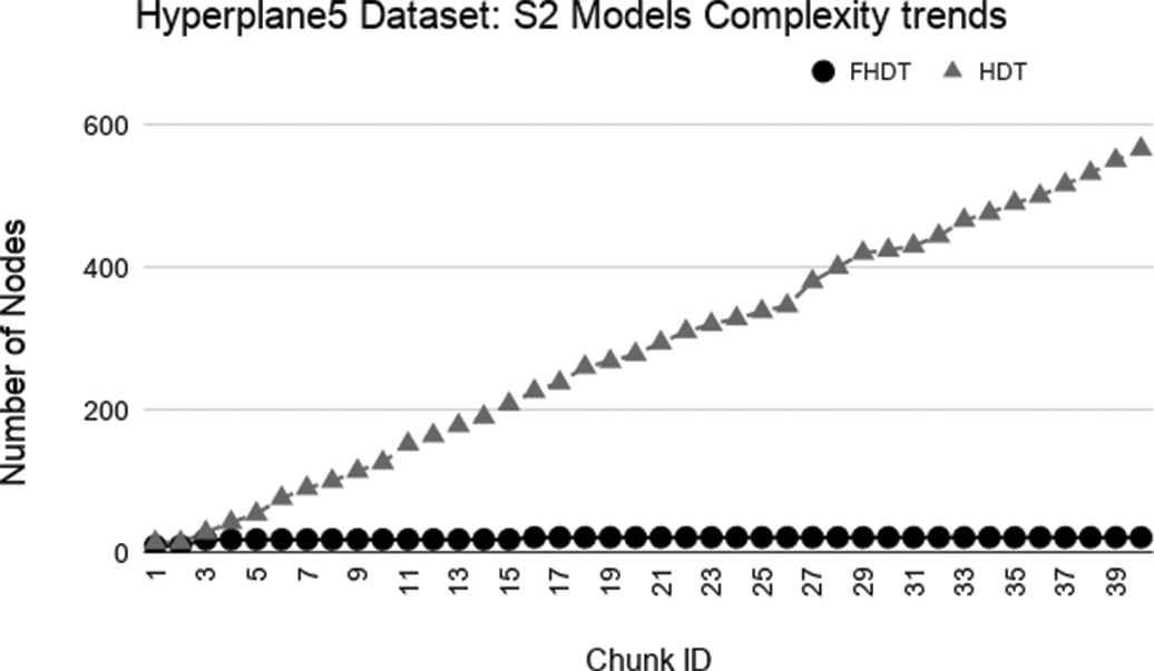
Model complexity trends for S2 on the Hyperplane5 dataset.
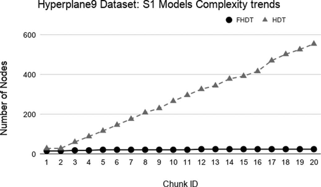
Model complexity trends for S1 on the Hyperplane9 dataset.
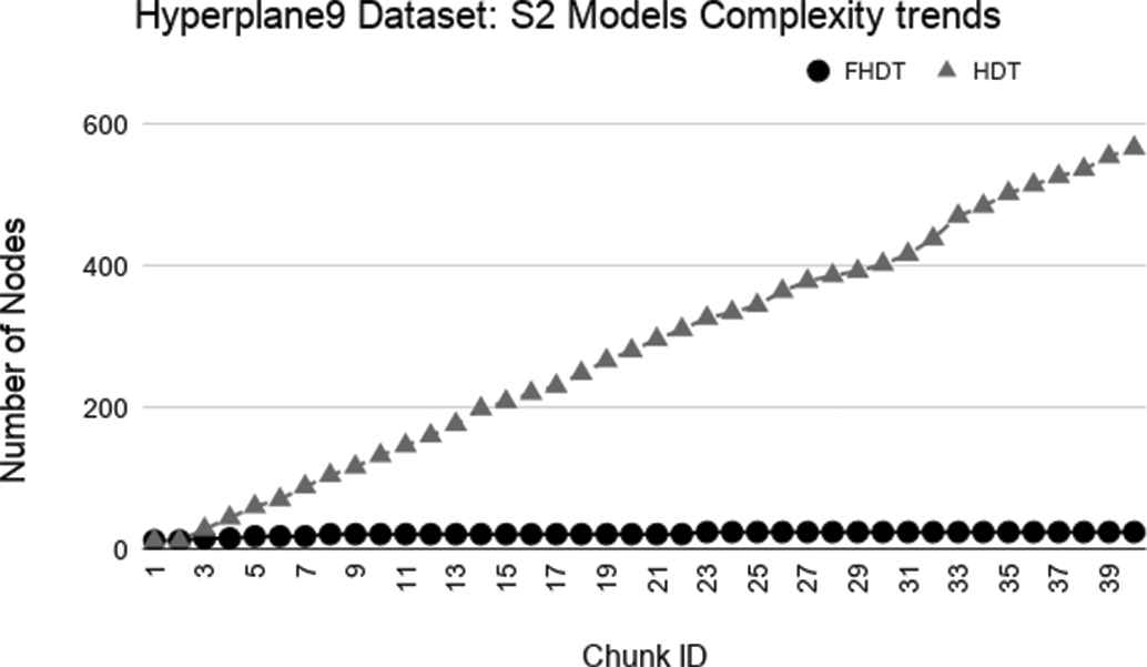
Model complexity trends for S2 on the Hyperplane9 dataset.
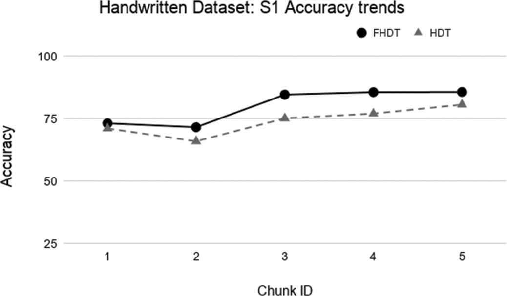
Test-the-train experiment: Accuracy trends for S1 on the Handwritten digits dataset.
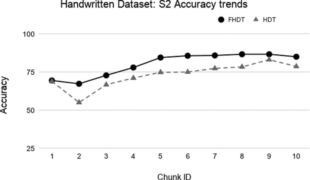
Test-the-train experiment: Accuracy trends for S2 on the Handwritten digits dataset.
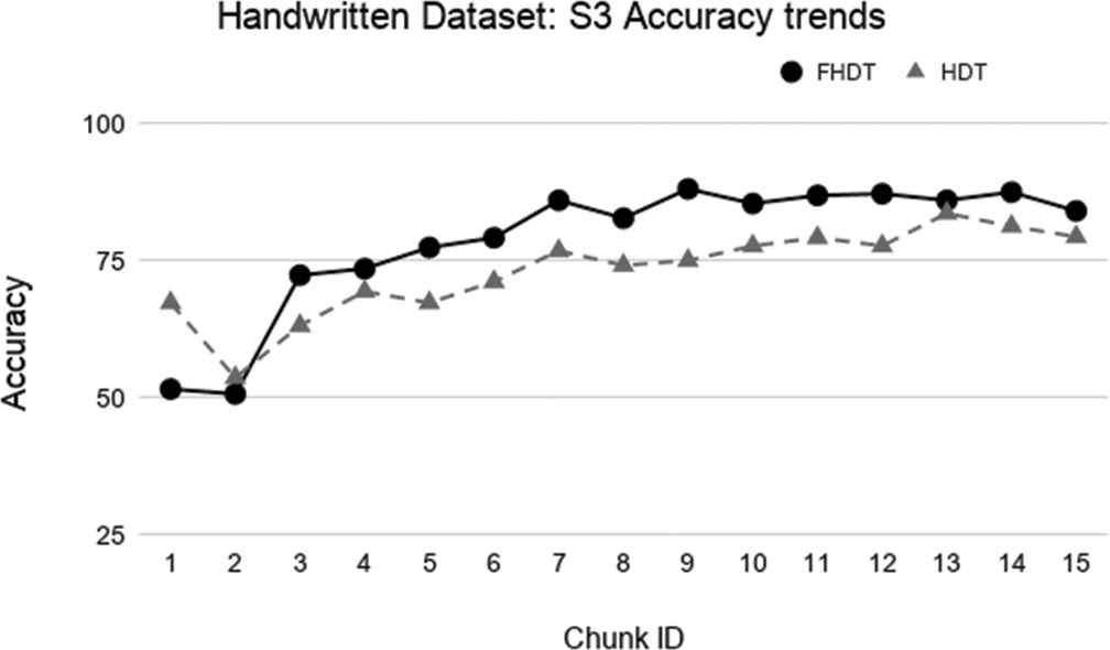
Test-the-train experiment: Accuracy trends for S3 on the Handwritten digits dataset.
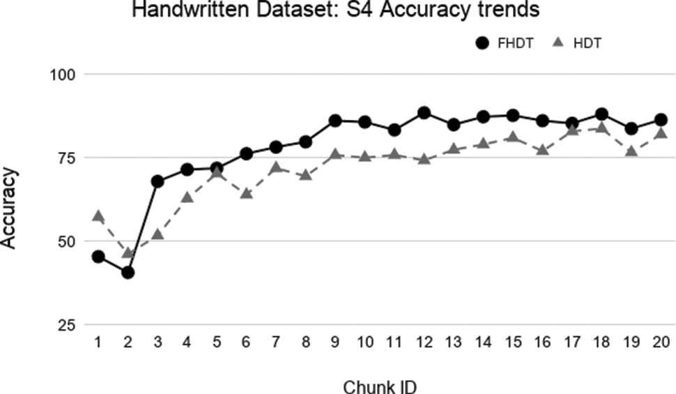
Test-the-train experiment: Accuracy trends for S4 on the Handwritten digits dataset.
The aforementioned figures clearly show that, in most cases, FHDT outperforms, in terms of accuracy, HDT. Specifically, FHDT outperforms HDT after analyzing one or two training chunks. It is worth noticing that, for this dataset, the two models do not suffer from the concept drift problem. Indeed, their accuracy increases while the number of training instances grows. This is also due to the fact that the classes are uniformly distributed in the chunks.
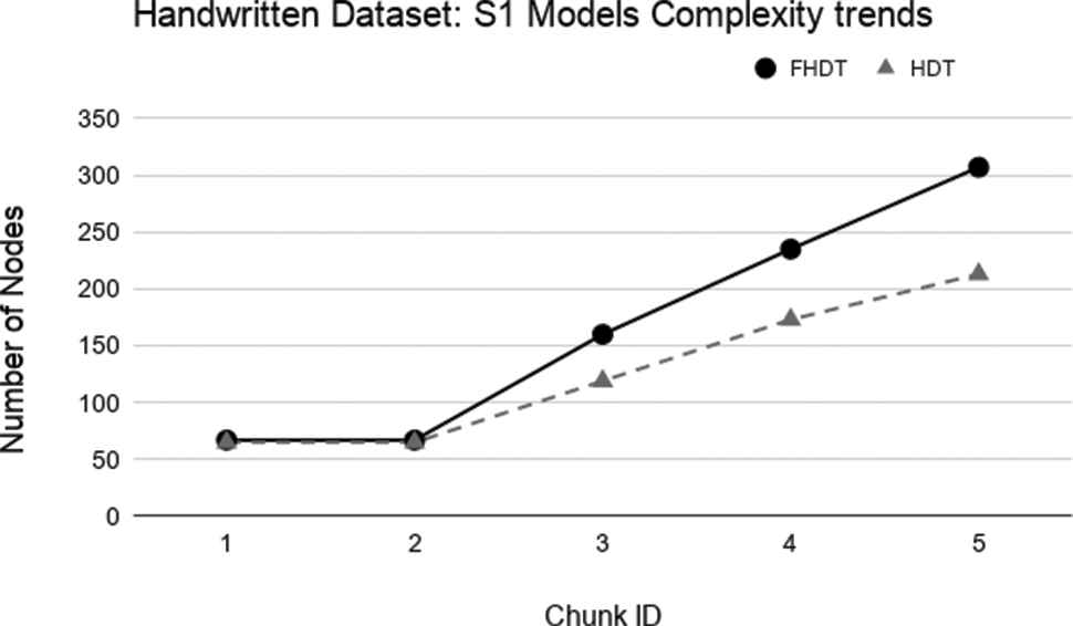
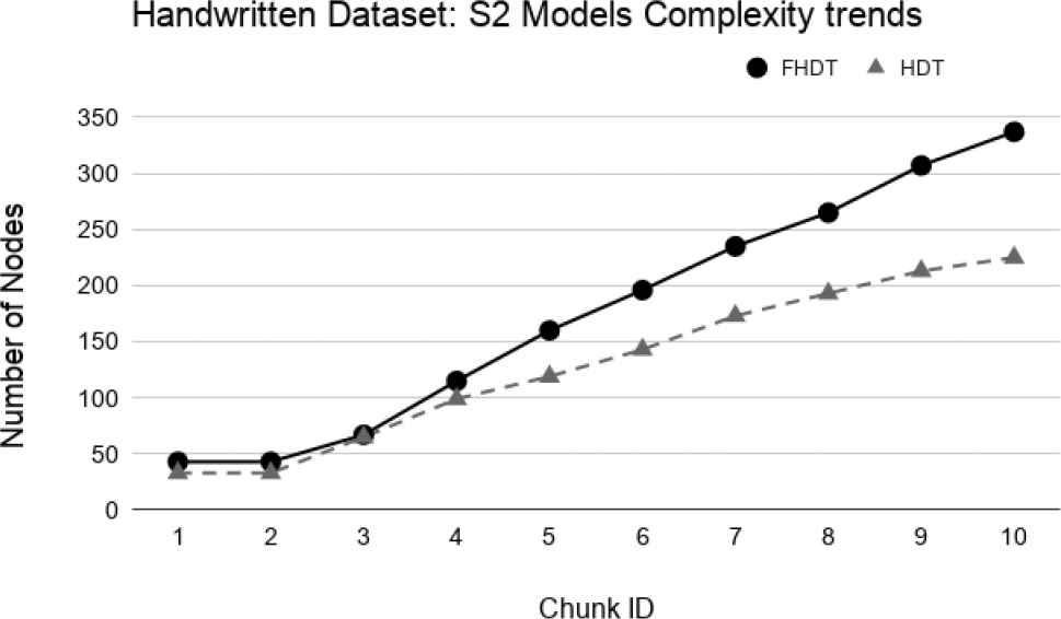
As regards the complexity of the models, Figures 19–22 show the trends of the number of nodes of each tree obtained by FHDT and HDT on S1, S2, S3, and S4, respectively, along the sequence of chunks. We can observe that the number of nodes in FHDT increases faster than in HDT. However, the increasing of the total number of nodes seems to be linear with the increasing of the chunks considered during the learning stage: the slope of FHDT is a bit greater than the one of HDT. Table 7 shows the accuracy, the depth expressed in terms of the number of levels, the number of nodes, and the number of leaves of the trees in the qth chunk.
Model complexity trends for S1 on the Handwritten digits dataset.
Model complexity trends for S2 on the Handwritten digits dataset.
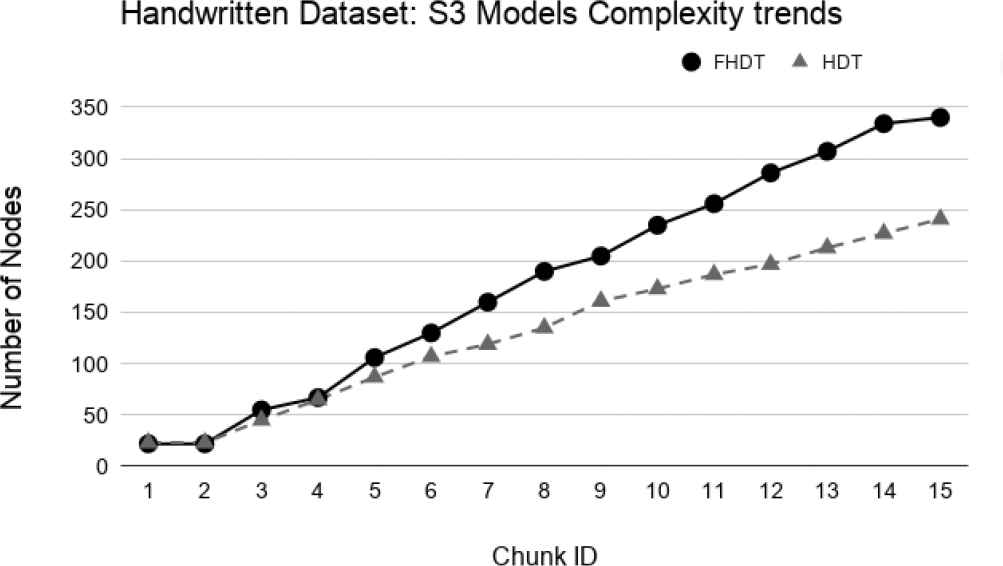
Model complexity trends for S3 on the Handwritten digits dataset.
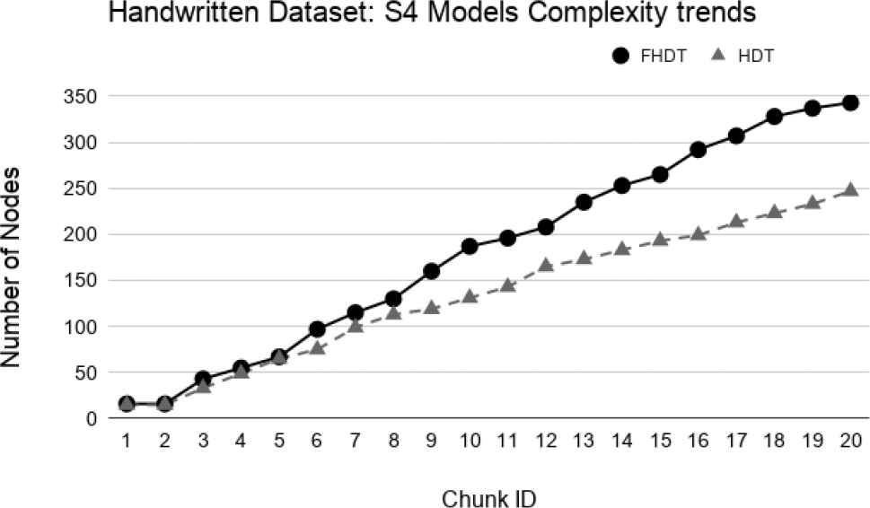
Model complexity trends for S4 on the Handwritten digits dataset.
Even though the models generated by the HDT learning procedure are more compact than the ones generated by the FHDT learning procedure, we have to consider that the rules that may be extracted from FHDT are characterized by a higher level of interpretability than the ones extracted from HDT. Indeed, the FHDT rules are expressed in linguistic terms easily understandable, while the HDT rules are based on numeric intervals. We will discuss some examples of rules in Section 5.4.2.
Figures 23–26 show the trends of the accuracy obtained by FHDT and HDT on S1, S2, S3, and S4, respectively along the sequence of chunks, considering the test set. We point out that the trends of the complexity of the models are the same as the ones shown in Figures 19–22. The results confirm that also on the test set, FHDT outperforms HDT in terms of achieved accuracy for all the different splitting strategies.
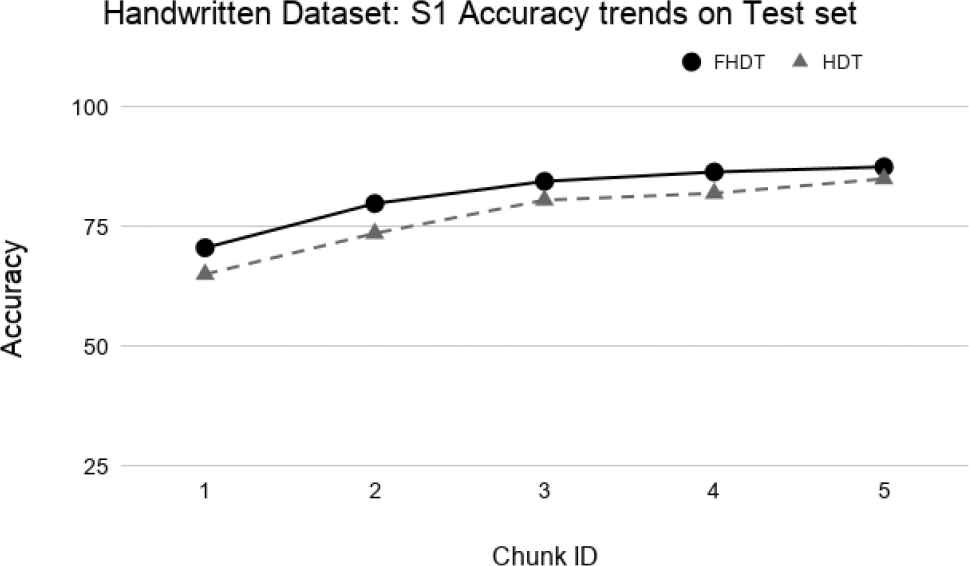
Test-the-test experiment: Accuracy trends for S1 on the Handwritten digits dataset.
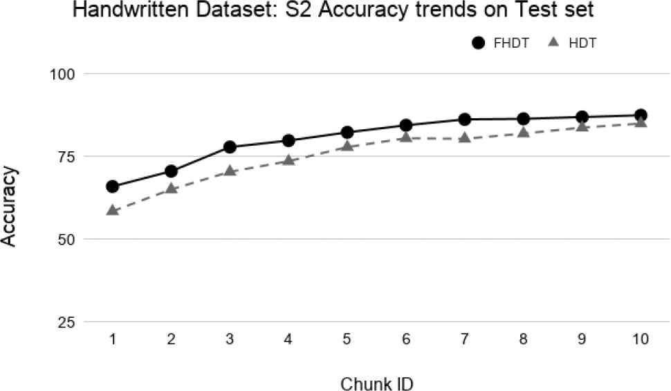
Test-the-test experiment: Accuracy trends for S2 on the Handwritten digits dataset.
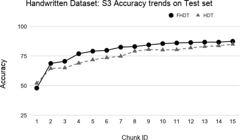
Test-the-test experiment: Accuracy trends for S3 on the Handwritten digits dataset.
| S1 |
FHDT |
HDT |
||||||
|---|---|---|---|---|---|---|---|---|
| Chunk ID | F-Measure | Depth | Nodes | Leaves | F-Measure | Depth | Nodes | Leaves |
| 1 | 0.883 | 2 | 7 | 5 | 0.830 | 8 | 61 | 31 |
| 17 | 0.837 | 2 | 7 | 5 | 0.817 | 18 | 917 | 459 |
| 25 | 0.861 | 2 | 7 | 5 | 0.836 | 19 | 1377 | 689 |
| 40 | 0.783 | 2 | 7 | 5 | 0.729 | 21 | 2267 | 1134 |
| 50 | 0.817 | 2 | 7 | 5 | 0.811 | 22 | 2827 | 1414 |
| S2 |
FHDT |
HDT |
||||||
|---|---|---|---|---|---|---|---|---|
| Chunk ID | F-Measure | Depth | Nodes | Leaves | F-Measure | Depth | Nodes | Leaves |
| 1 | 0.896 | 2 | 7 | 5 | 0.893 | 6 | 29 | 15 |
| 25 | 0.794 | 2 | 7 | 5 | 0.770 | 17 | 725 | 363 |
| 50 | 0.810 | 2 | 7 | 5 | 0.774 | 19 | 1445 | 723 |
| 75 | 0.796 | 2 | 7 | 5 | 0.718 | 20 | 2161 | 1081 |
| 100 | 0.822 | 2 | 7 | 5 | 0.819 | 22 | 2849 | 1425 |
Results for some relevant chunks of the SEA dataset.
| S1 |
FHDT |
HDT |
||||||
|---|---|---|---|---|---|---|---|---|
| Chunk ID | F-Measure | Depth | Nodes | Leaves | F-Measure | Depth | Nodes | Leaves |
| 1 | 0.841 | 3 | 19 | 13 | 0.733 | 8 | 29 | 15 |
| 10 | 0.830 | 4 | 22 | 15 | 0.735 | 16 | 295 | 148 |
| 20 | 0.837 | 4 | 22 | 15 | 0.777 | 18 | 551 | 276 |
| S2 |
FHDT |
HDT |
||||||
|---|---|---|---|---|---|---|---|---|
| Chunk ID | F-Measure | Depth | Nodes | Leaves | F-Measure | Depth | Nodes | Leaves |
| 1 | 0.876 | 2 | 10 | 7 | 0.772 | 6 | 15 | 8 |
| 20 | 0.868 | 4 | 22 | 15 | 0.732 | 16 | 279 | 140 |
| 40 | 0.864 | 4 | 22 | 15 | 0.740 | 18 | 567 | 284 |
Results for some relevant chunks of the Hyperplane5 dataset.
| S1 |
FHDT |
HDT |
||||||
|---|---|---|---|---|---|---|---|---|
| Chunk ID | F-Measure | Depth | Nodes | Leaves | F-Measure | Depth | Nodes | Leaves |
| 1 | 0.893 | 3 | 16 | 11 | 0.792 | 8 | 29 | 15 |
| 10 | 0.778 | 4 | 22 | 15 | 0.660 | 17 | 267 | 134 |
| 20 | 0.746 | 4 | 25 | 17 | 0.720 | 19 | 555 | 278 |
| S2 |
FHDT |
HDT |
||||||
|---|---|---|---|---|---|---|---|---|
| Chunk ID | F-Measure | Depth | Nodes | Leaves | F-Measure | Depth | Nodes | Leaves |
| 1 | 0.876 | 2 | 13 | 9 | 0.774 | 6 | 13 | 7 |
| 20 | 0.760 | 4 | 22 | 15 | 0.670 | 17 | 281 | 141 |
| 40 | 0.720 | 4 | 25 | 17 | 0.706 | 20 | 567 | 284 |
Results for some relevant chunks of the Hyperplane9 dataset.
| Splitting |
FHDT |
HDT |
||||||
|---|---|---|---|---|---|---|---|---|
| Accuracy | Depth | Nodes | Leaves | Accuracy | Depth | Nodes | Leaves | |
| S1 | 85.74 | 8 | 307 | 207 | 80.69 | 6 | 213 | 107 |
| S2 | 85.11 | 8 | 337 | 225 | 78.76 | 6 | 233 | 117 |
| S3 | 84.11 | 8 | 340 | 227 | 79.41 | 6 | 241 | 121 |
| S4 | 86.45 | 8 | 343 | 249 | 82.07 | 6 | 247 | 124 |
Results for the models obtained in the last training chunk on the Handwritten digits dataset.
| S1 |
|||
|---|---|---|---|
| Ch ID | Time Slot | % not occupied | % occupied |
| 1 | 2015-02-04 17:51:00–2015-02-04 23:58:59 | 95.66% | 4.34% |
| 2 | 2015-02-05 00:00:00–2015-02-05 23:58:59 | 62.57% | 37.43% |
| 3 | 2015-02-06 00:00:00–2015-02-06 23:58:59 | 59.31% | 40.69% |
| 4 | 2015-02-07 00:00:00–2015-02-07 23:58:59 | 100% | 0% |
| 5 | 2015-02-08 00:00:00–2015-02-08 23:58:59 | 100% | 0% |
| 6 | 2015-02-09 00:00:00–2015-02-09 23:58:59 | 62.92% | 37.08% |
| 7 | 2015-02-10 00:00:00–2015-02-10 09:33:00 | 90.59% | 9.41% |
| S2 |
|||
|---|---|---|---|
| Ch ID | Time Slot | % not occupied | % occupied |
| 1 | 2015-02-04 17:51:00–2015-02-04 23:58:59 | 95.66% | 4.34% |
| 2 | 2015-02-05 00:00:00–2015-02-05 11:58:59 | 64.72% | 35.28% |
| 3 | 2015-02-05 12:00:00–2015-02-05 23:58:59 | 60.42% | 39.58% |
| 4 | 2015-02-06 00:00:00–2015-02-06 11:58:59 | 65.56% | 34.44% |
| 5 | 2015-02-06 12:00:00–2015-02-06 23:58:59 | 53.06% | 46.94% |
| 6 | 2015-02-07 00:00:00–2015-02-07 11:58:59 | 100% | 0% |
| 7 | 2015-02-07 12:00:00–2015-02-07 23:58:59 | 100% | 0% |
| 8 | 2015-02-08 00:00:00–2015-02-08 11:58:59 | 100% | 0% |
| 9 | 2015-02-08 12:00:00–2015-02-08 23:58:59 | 100% | 0% |
| 10 | 2015-02-09 00:00:00–2015-02-09 11:58:59 | 73.33% | 26.67% |
| 11 | 2015-02-09 12:00:00–2015-02-09 23:58:59 | 52.5% | 47.5% |
| 12 | 2015-02-10 00:00:00–2015-02-10 09:33:00 | 90.59% | 9.41% |
| S3 |
|||
|---|---|---|---|
| Ch ID | Time Slot | % not occupied | % occupied |
| 1 | 2015-02-04 17:51:00–2015-02-04 23:58:59 | 95.66% | 4.34% |
| 2 | 2015-02-05 00:00:00–2015-02-05 07:59:59 | 95.84% | 4.16% |
| 3 | 2015-02-05 08:00:59–2015-02-05 15:59:00 | 17.75% | 82.25% |
| 4 | 2015-02-05 16:00:00–2015-02-05 23:58:59 | 73.96% | 26.04% |
| 5 | 2015-02-06 00:00:00–2015-02-06 07:59:59 | 97.3% | 2.7% |
| 6 | 2015-02-06 08:00:59–2015-02-06 15:59:00 | 6.89% | 93.11% |
| 7 | 2015-02-06 16:00:00–2015-02-06 23:58:59 | 73.54% | 26.46% |
| 8 | 2015-02-07 00:00:00–2015-02-07 07:59:59 | 100% | 0% |
| 9 | 2015-02-07 08:00:59–2015-02-07 15:59:00 | 100% | 0% |
| 10 | 2015-02-07 16:00:00–2015-02-07 23:58:59 | 100% | 0% |
| 11 | 2015-02-08 00:00:00–2015-02-08 07:59:59 | 100% | 0% |
| 12 | 2015-02-08 08:00:59–2015-02-08 15:59:00 | 100% | 0% |
| 13 | 2015-02-08 16:00:00–2015-02-08 23:58:59 | 100% | 0% |
| 14 | 2015-02-09 00:00:00–2015-02-09 07:59:59 | 100% | 0% |
| 15 | 2015-02-09 08:00:59–2015-02-09 15:59:00 | 14.61% | 85.39% |
| 16 | 2015-02-09 16:00:00–2015-02-09 23:58:59 | 73.96% | 26.04% |
| 17 | 2015-02-10 00:00:00–2015-02-10 09:33:00 | 90.59% | 9.41% |
Class distribution for the Occupancy dataset in S1, S2, and S3.
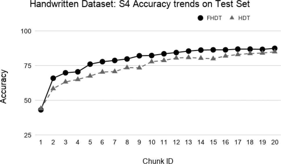
Test-the-test experiment: Accuracy trends for S4 on the Handwritten digits dataset.
5.4.2. Occupancy dataset
As already mentioned, this dataset reflects a real application of a Smart Building, in which an intelligent system can be involved in the automatic management of electricity consumption of appliances and devices. We can envision such a system mainly composed of a sensing module, an occupancy estimation module, and an automation module. The sensing module continuously gets measures from sensors and feeds the estimation module, which provides an output about the occupancy or not of a specific room. The automation module is in charge of switching off devices and appliances, if the room is empty. In Table 8, we show the distribution of the classes into the instances composing each chunk for S1, S2, and S3, respectively. In the table, the Ch ID header stands for the ID of the data chunk.
One can notice that the class distribution changes in the chunks. Changes in class distribution are more appreciable when we consider a finer granularity. We observe that in S1, S2, and S3, the splitting interval consists of 24, 12, and 8 hours, respectively. Moreover, February 7th and 8th, 2015 were public holidays, thus the room was always not occupied by people, as it also occurs during night hours. Thus, we expect that the incremental classifiers will experience a concept drift issue, especially when the number of chunks increases.
Since we are dealing with a binary and imbalanced dataset, we evaluate the performance of the classifiers in terms of F-measure of the relevant class, namely the non-occupied one. Indeed, in a smart building framework, it will be more interesting to identify empty rooms in order to automatically switch off all power consuming devices and appliances. However, we also extracted the values of precision and recall for each class. The trends of such measures are very similar to those of the F-measure for the relevant class, thus, for the sake of brevity, we skipped to show them.
As regards the test-the-train experiments, in Figures 27–29, we show the trends of the F-measure obtained by FHDT and HDT on, respectively, S1, S2, and S3 along the sequence of chunks. It is worth noticing that for the first chunk we show the F-measure calculated considering the chunk as training and test set. For the remaining chunks, we show the F-measure calculated considering each chunk q as test set, after an incremental learning process which includes training samples till chunk q − 1.
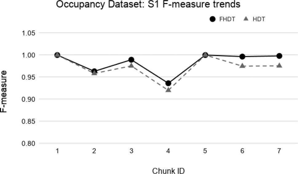
Test-the-train experiment: F-measure trends for S1 on the Occupancy dataset.
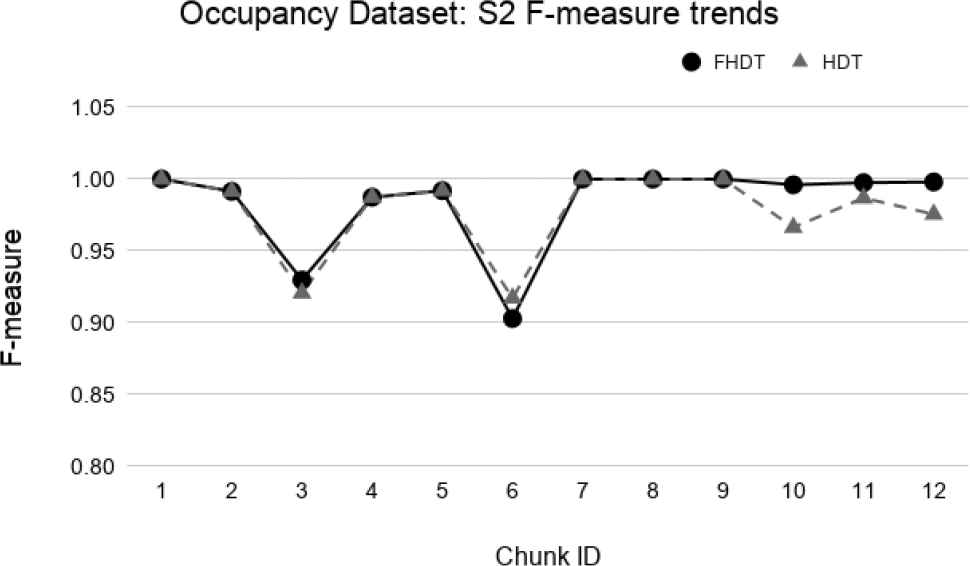
Test-the-train experiment: F-measure trends for S2 on the Occupancy dataset.
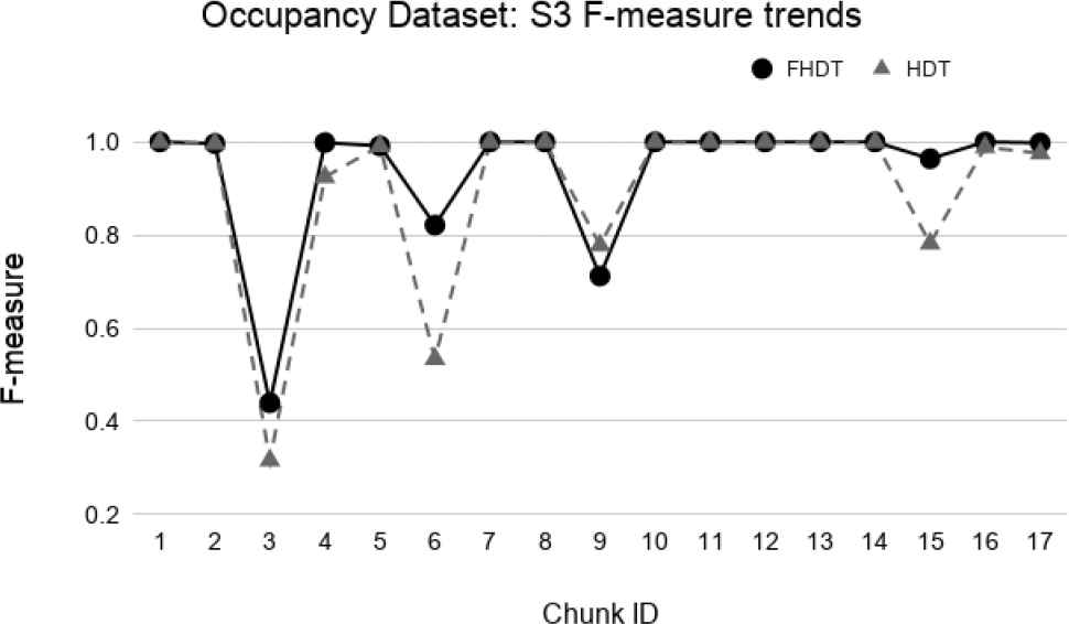
Test-the-train experiment: F-measure trends for S3 on the Occupancy dataset.
We observe that, in most of the time intervals, the F-measure achieved by FHDT is higher than the one achieved by HDT. The better classification performance of FHDT is much more evident in the last chunks and especially in S3, when the concept drift is, as expected, much more visible.
Figures 30–32 show the trends of the number of nodes for the two compared incremental decision trees. Unlike the Handwritten dataset, we highlight that the size of FHDT grows much more slowly than the one of HDT. Moreover, after using all the chunks for the training stage, the number of nodes composing the HDT is more than 3 times higher than the one of FHDT (53 nodes vs 16 nodes, respectively). After the last training chunk, the final numbers of leaves of the trees are equal to 11 and 27 for FHDT and HDT, respectively. It is worth to highlight that, after the last training chunk, when the entire training set has been shown to the learning algorithm, the generated trees, both FHDT and HDT, have the same structure for S1, S2, and S3. In conclusion, for the Occupancy dataset, we can state that the models, incrementally generated by the FHDT learning procedure are always characterized by a lower complexity level than the ones generated by the HTD learning procedure.
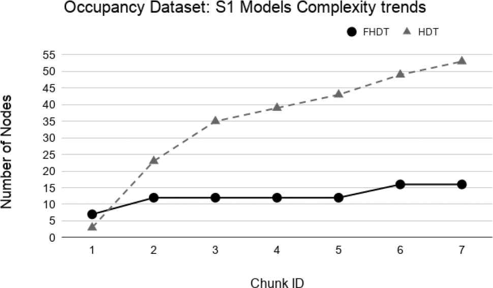
Models complexity trends for S1 on the Occupancy dataset.
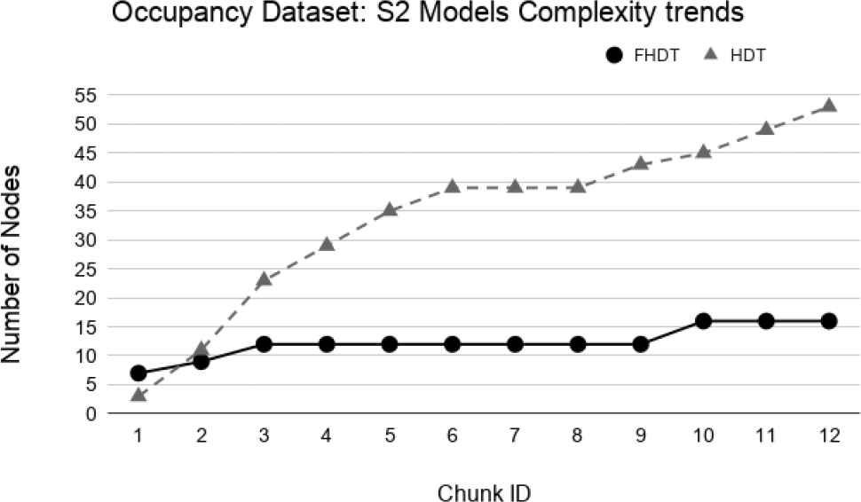
Models complexity trends for S2 on the Occupancy dataset.
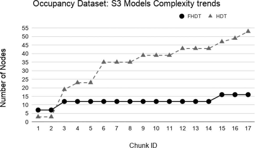
Models complexity trends for S3 on the Occupancy dataset.
In order to highlight the high interpretability level associated with models generated by the FHDT learning, in Figure 33 we show the FHDT obtained after feeding the incremental learning process with the entire training set. We labeled the fuzzy sets, adopted in the partitioning of the input attributes, as “Low,” “Medium,” and “High.” As a consequence of the rules, we considered the class with the highest weight in the specific leaf.
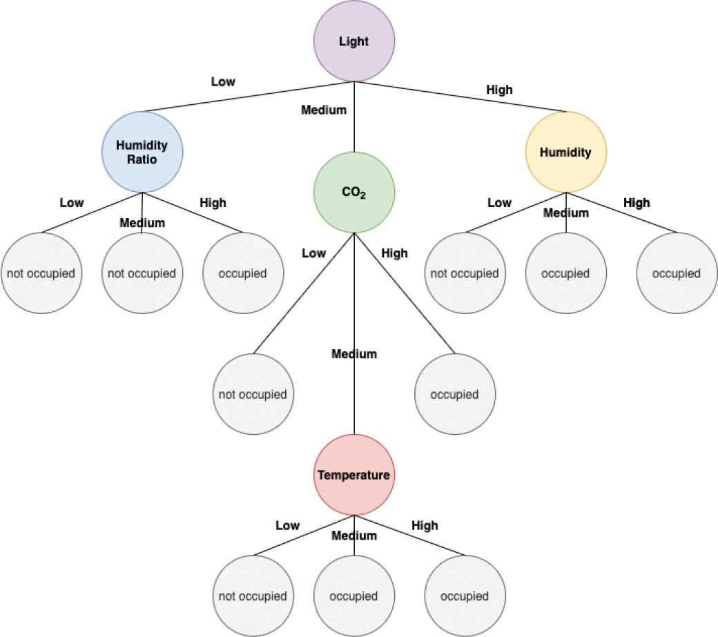
Final FHDT for the Occupancy dataset.
As we can see, the model itself is very readable, far from being a black box like some classical machine learning models, such as neural networks and support vector machines. Moreover, unlike the trees generated by the HDT learning, it is possible to extract linguistic rules, which can help the user to understand how a specific output has been obtained. In the following, we show a couple of examples of the obtained fuzzy rules, extracted from the generated FHDT.
R1 : IF Light is Low AND HumidityRatio is Low
THEN Room is not occupied
R2 : IF Light is Medium AND CO2 is High
THEN Room is occupied
Moreover, we recall that defining fuzzy partitions for each attribute, and consequently generating fuzzy rules, allows adequately handling noisy and vague data that may be extracted from the sensors deployed in the room. Conversely, this capability is missing in classical decision trees, which take decisions considering crisp rules such as the one shown in the following:
R1 : IF Light is ⩽ 0.34 AND HumidityRatio is ⩽ 0.030
THEN Room is not occupied
Finally, for the test-the-train experiments, an excerpt of the results, in terms of classification performance and of complexity of the models, is presented in Table 9. Specifically, we show the results for the chunks which are characterized by the most evident concept drift.
Figures 34–39 show the trends of the F-measure of the relevant class, for both FHDT and HDT, calculated on Test 1 and Test 2 datasets, respectively. We recall that the trends of the complexity of the models are the same as the ones shown in Figures 30–32. Indeed, for the test-the-test experiments, the models are incrementally trained on the same data chunks as those adopted for the test-the-train experiments. As regards the classification performance, for the test-the-test experiments, the results confirm that FHDT always outperforms HDT, even with the lowest complexity levels of the models. Notice that for both FHDT and HDT, the values of F-measure remain more or less constant along the time intervals. However, after the initial training chunks, as regards HDT classification performance, F-measure decreases for Test 1 and slightly increases for Test2.
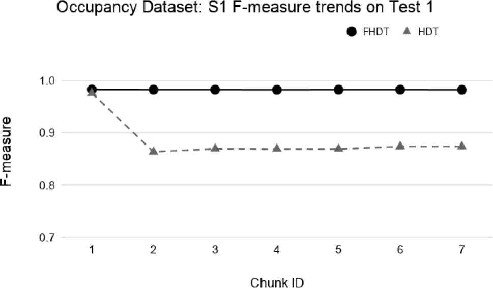
Test-the-test experiment: F-measure trends for S1 on the Occupancy Test1.
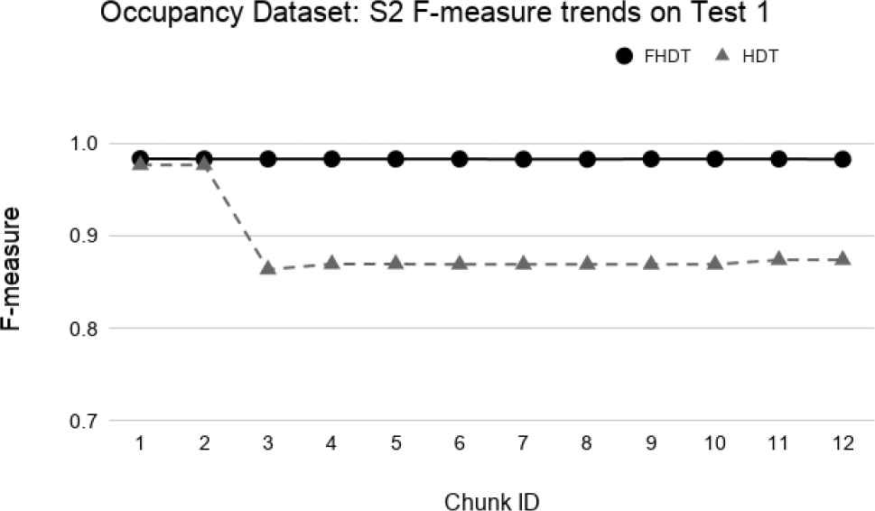
Test-the-test experiment: F-measure trends for S2 on the Occupancy Test1.
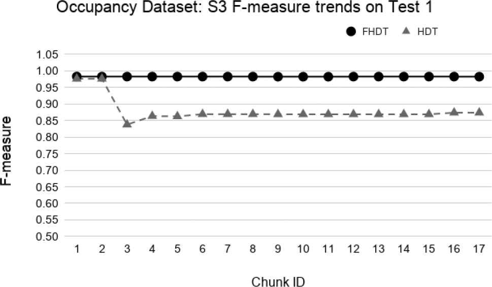
Test-the-test experiment: F-measure trends for S3 on the Occupancy Test1.
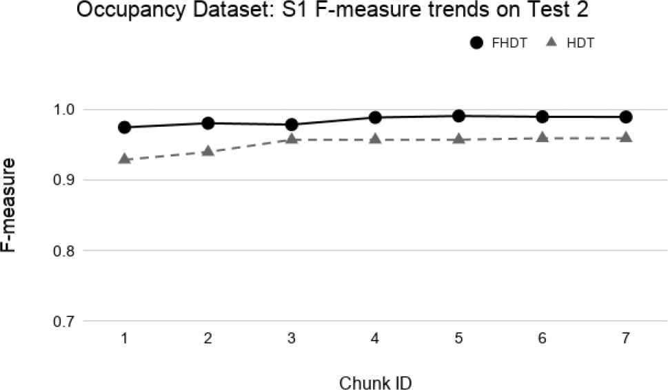
Test-the-test experiment: F-measure trends for S1 on the Occupancy Test2.
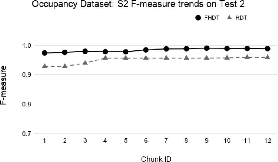
Test-the-test experiment: F-measure trends for S2 on the Occupancy Test2.
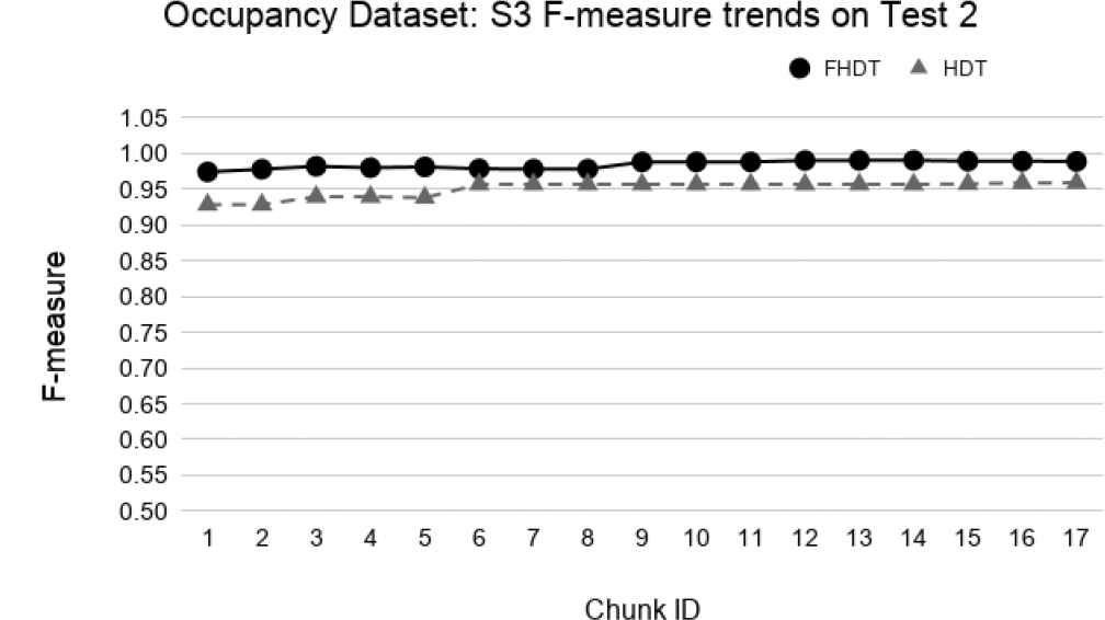
Test-the-test experiment: F-measure trends for S3 on the Occupancy Test2.
| S1 |
FHDT |
HDT |
||||||
|---|---|---|---|---|---|---|---|---|
| Chunk ID | F-Measure | Depth | Nodes | Leaves | F-Measure | Depth | Nodes | Leaves |
| 3 | 0.989 | 3 | 13 | 9 | 0.975 | 7 | 35 | 18 |
| 4 | 0.936 | 3 | 13 | 9 | 0.920 | 7 | 39 | 20 |
| 6 | 0.996 | 3 | 16 | 11 | 0.974 | 7 | 49 | 25 |
| 7 | 0.997 | 3 | 16 | 11 | 0.975 | 7 | 53 | 27 |
| S2 |
FHDT |
HDT |
||||||
|---|---|---|---|---|---|---|---|---|
| Chunk ID | F-Measure | Depth | Nodes | Leaves | F-Measure | Depth | Nodes | Leaves |
| 3 | 0.929 | 2 | 13 | 9 | 0.920 | 7 | 23 | 12 |
| 6 | 0.902 | 3 | 13 | 9 | 0.917 | 7 | 39 | 20 |
| 11 | 0.997 | 3 | 16 | 11 | 0.986 | 7 | 49 | 25 |
| 12 | 0.997 | 3 | 16 | 11 | 0.975 | 7 | 53 | 27 |
| S3 |
FHDT |
HDT |
||||||
|---|---|---|---|---|---|---|---|---|
| Chunk ID | F-Measure | Depth | Nodes | Leaves | F-Measure | Depth | Nodes | Leaves |
| 3 | 0.439 | 2 | 13 | 9 | 0.316 | 1 | 19 | 10 |
| 5 | 0.991 | 3 | 13 | 9 | 0.991 | 7 | 23 | 12 |
| 8 | 1 | 3 | 13 | 9 | 1 | 7 | 35 | 18 |
| 14 | 1 | 3 | 13 | 9 | 1 | 7 | 43 | 22 |
| 17 | 0.997 | 3 | 16 | 11 | 0.975 | 7 | 53 | 27 |
Results for some relevant chunks of the Occupancy dataset.
Finally, continuing the discussion on the test-the-test experiments, in Table 10, we show a comparison of the results achieved by FHDT and HDT with the recent DISSFCM algorithm [19], proposed for classifying data streams, and with other classical batch classifiers. Actually, in this case, similar to the analysis performed in Ref. [19], we calculated the average values of the accuracy of each trend for S1, S2, and S3, and compared them with the average values of accuracy extracted from the paper in which DISSFCM has been experimented on the Occupancy dataset. In Ref. [19] the authors compared, in terms of average accuracy, DISSFCM with other classical batch classifiers, namely Random Forest (RF), Gradient Boosting Machines (GBM), Linear Discriminant Analysis (LDA), and Classification and Regression Trees (CART). We recall that for these batch classifiers, the entire training set has been provided as input for the learning algorithm, thus for them, we do not have the experiments on S1, S2, and S3. The results confirm that FHDT always outperforms HDT and DISSFCM, for S1, S2, and S3, on both Test 1 and Test2. As regards the comparison with batch classifiers, LDA always achieves the highest average accuracy. However, the average accuracies obtained by FHDT are only about 1% lower than those obtained by LDA, which is, unlike FHDT, a black box classification model.
| Model | Test 1 | Test 2 |
|---|---|---|
| FHDT (S1) | 97.85 | 97.56 |
| HDT (S1) | 83.76 | 92.21 |
| DISSFCM (S1) | 95.34 | 93.83 |
| FHDT (S2) | 97.85 | 97.51 |
| DISSFCM (S2) | 94.59 | 90.63 |
| HDT (S2) | 84.08 | 92.24 |
| FHDT (S3) | 97.85 | 97.58 |
| HDT (S3) | 82.94 | 92.12 |
| DISSFCM (S3) | 94.86 | 89.68 |
| RF | 95.05 | 97.16 |
| GBM | 93.06 | 95.14 |
| CART | 95.57 | 96.47 |
| LDA | 97.90 | 98.76 |
Average accuracy comparison for the Test-the-test experiments.
5.5. Execution Time Analysis of the Incremental Learning Algorithms
Table 11 shows, for each considered dataset, the time (in seconds) needed for analyzing the entire stream of data by the incremental learning algorithms for building both FHDTs and HDTs. As regards the real-world datasets, we considered only the training set as the entire stream of data. In the table, the first three columns contain the name of the dataset, the number of instances, and the number of attributes, respectively, which characterize each data stream, whereas the last two columns contain the execution times of the incremental learning algorithms for FHDT and HDT, respectively.
| Dataset | #Instances | #Attributes | FHDT | HDT |
|---|---|---|---|---|
| SEA | 60000 | 3 | 2.60 | 0.18 |
| Hyperplane5 | 10000 | 10 | 6.48 | 0.11 |
| Hyperplane9 | 10000 | 10 | 8.35 | 0.17 |
| Handwritten | 5058 | 64 | 4.34 | 0.11 |
| Occupancy | 8143 | 5 | 4.71 | 0.07 |
Execution times (in s) of the incremental learning algorithms.
We observe that the HDT and FHDT learning algorithms require less than 0.2 seconds and up to 8.35 seconds for building the decision tree, respectively. Thus, the execution time for learning FHDTs is one order of magnitude higher than the execution time for learning HDTs. This is mainly due to the fact that, as discussed in Section 3.2, each training instance may activate simultaneously multiple paths in FHDT and several matching degrees must be calculated for updating the statistics of the decision nodes and for checking the splitting conditions.
6. CONCLUSION AND FUTURE WORK
In this paper, we have presented FHDT, the fuzzy version of the traditional Hoeffding Tree (HDT) for data stream classification. More precisely, we have defined for each input attribute a fuzzy strong uniform partition and have taken advantage of the FIG as a metric to choose the best input attribute in order to split decision nodes. Furthermore, we have modified the Hoeffding bound to take into consideration that one instance can belong to different leaves with different membership degrees.
We have experimented the proposed FHDT learning procedure on three synthetic datasets, usually adopted for analyzing concept drifts in data stream classification, and on two real-world datasets, already exploited in some recent researches on fuzzy systems for streaming data. The data streams have been simulated by splitting the datasets in chunks. We have compared the obtained results achieved by FHDT with the ones achieved by HDT in terms of accuracy, complexity, and computational time. Moreover, as regards the real dataset related to the detection of the presence or absence of persons in a room, we have also shown some comparisons with a recent streaming data classification algorithm, based on fuzzy clustering, and with some state-of-the-art machine learning algorithms. The results have demonstrated that the FHDTs generated by the learning procedure proposed in this paper outperform the HDTs in terms of classification performance and complexity, although the time needed to learn them is longer than the one needed to learn the HDTs. We have shown some examples of linguistic fuzzy rules, that can be extracted from an FHDT: these rules result to be more interpretable, and also more suitable for handling data vagueness, than the ones that can be extracted from an HDT.
Future work may regard the design, the implementation, and the experimentation of an incremental learning algorithm for FDT in a distributed computing framework for Big Data. Moreover, we envision to adopt the FHDT learning algorithm in an IoT architecture for anomaly detection and predictive maintenance for Industry 4.0.
CONFLICTS OF INTEREST
The authors declare that they have no competing interests.
AUTHORS' CONTRIBUTIONS
The study was conceived and designed by Prof. Pietro Ducange supervised by Prof. Francesco Marcelloni. The implementation and experiments have been performed by Dr. Riccardo Pecori. All authors contributed in writing, proofreading, and approving the manuscript.
ACKNOWLEDGMENTS
The contribution to this work of Prof. Pietro Ducange and Prof. Francesco Marcelloni has been supported by the Italian Ministry of Education and Research (MIUR), in the framework of the CrossLab project (Departments of Excellence). The work of Dr. Riccardo Pecori has been supported by the PON R&I 2014-2020 “AIM: Attraction and International Mobility” project, funded by the Italian Ministry of Education and Research (MIUR), the European Social Fund, and the European Regional Development Fund.
DATA AVAILABILITY STATEMENT
The datasets adopted in this study are available in the UCI repository, at https://archive.ics.uci.edu/ml/datasets.php and at https://www.win.tue.nl/~mpechen/data/DriftSets/.
Footnotes
REFERENCES
Cite this article
TY  - JOUR
AU  - Pietro Ducange
AU  - Francesco Marcelloni
AU  - Riccardo Pecori
PY  - 2021
DA  - 2021/02/23
TI  - Fuzzy Hoeffding Decision Tree for Data Stream Classification
JO  - International Journal of Computational Intelligence Systems
SP  - 946
EP  - 964
VL  - 14
IS  - 1
SN  - 1875-6883
UR  - https://doi.org/10.2991/ijcis.d.210212.001
DO  - 10.2991/ijcis.d.210212.001
ID  - Ducange2021
ER  -