
Slope Sliding Force Prediction via Belief Rule-Based Inferential Methodology
 , Pan Liu1, Feng Ma2, Chengrong Ma3, Zhigang Tao4, 5, *
- DOI
- 10.2991/ijcis.d.210216.001How to use a DOI?
- Keywords
- Slope landslide; Sliding force; Belief rule base; SLP optimization algorithm; West–East Gas Pipeline Project
- Abstract
Slope sliding force can be measured by an anchor cable sensor with the negative Poisson's ratio (NPR) property. It is capable of reflecting the stability of the slope intuitively. Thus, predicting the variation trend of the sliding force is able to achieve early warning for landslide disaster, thereby avoiding losses to the lives and property of the people. In this paper, due to the uncertain variation of the sliding force, a belief rule-based (BRB) sliding force prediction model is established to describe the nonlinear and uncertain relationship between the history/current sliding force and the future sliding force. In this model, the activated belief rules are fused by adopting the evidence reasoning (ER) algorithm. And based on the fused results, the sliding force at a future time can be predicted accurately. Moreover, considering the variation of the sliding force on different slopes or different monitoring points in the same slope, a parameter transfer strategy of BRB model together with a corresponding online update method are proposed to achieve the adaptive design of the BRB prediction model. Finally, the effectiveness of the proposed sliding force prediction methods has been verified by experiments on the sub-section of the China West–East Gas Pipeline Project.
- Copyright
- © 2021 The Authors. Published by Atlantis Press B.V.
- Open Access
- This is an open access article distributed under the CC BY-NC 4.0 license (http://creativecommons.org/licenses/by-nc/4.0/).
1. INTRODUCTION
Slope landslides occur when sliding forces are greater than anti-sliding forces. It causes disasters, such as destroying railway and road traffic, damaging farmland and forests, destroying factories and mines, even drowning villages, which threaten people's lives and property. Normally, methods such as lidar technology [1], grating sensor technology [2], rainfall monitoring [3], groundwater level monitoring [4], are adopted to achieve early warning of slope landslides. However, these methods forecast landslides only by monitoring displacements and cracks [5], whereas the occurrence of the displacements and cracks does not necessarily cause landslides. Therefore, it is difficult for such methods to achieve accurate predictions.
Nevertheless, sliding forces are capable of reflecting the current state of the sliding body accurately. And the stability of slopes can be judged intuitively by measuring the sliding forces [6]. Thus, predicting the sliding forces is of great significance for early warning of disasters, so as to keep people's lives and property from damage. Moreover, research on predicting sliding forces is drawing more and more attention. Specifically, He et al. [7] developed a sliding force monitoring system based on a giant negative Poisson's ratio (NPR) anchor cable. In the system, a complex mechanical system is constructed by inserting a special artificial mechanical system into an unmeasured natural mechanical system [8, 9]. Bai et al. [10] used BP neural network to predict the slope stability of open-pit mine, and meanwhile pointed out that BP neural network is prone to fall into the local minimum. Li et al. [11] established a deformation and displacement prediction model of open-pit mine slope based on SVM, but the sensitivity of model parameters has not been further studied. Wang et al. [12] constructed a GM model-based on the Kalman filter to predict the deformation of highway slopes, but due to the complexity and mutability of highway slope deformation, the prediction accuracy was deficient. Sun et al. [13] proposed a monitoring and warning method of landslides in Pingzhuang West open-pit coal mine. The proposed method adopts the sliding remote monitoring and warning system which integrated the function of landslide reinforcement, detection, and warning, thereby realizing the whole process of slide force perception, transmission, analysis, monitoring, and warning. Tao et al. [14] adopt the plane polar projection method to analyze the landslide mechanism and use FLAC3D to build an NPR numerical analysis model which is used to make an early warning. However, the method cannot accurately grasp the magnitude of the sliding force at any time, and cannot be used for different slope migration and conversion.
At present, various sliding force monitoring and forecasting technologies have been successfully applied on 381 sites of 16 provinces across China, which involve slope monitoring on ancient landslides, high and steep loess natural slopes, urban construction slopes, open-pit coal mining, metal mining, highway project, and the West–East Gas Pipeline Project. Meanwhile, short-term and imminent warnings are able to be delivered after nearly ten years of sliding force monitoring and forecasting practice [15]. To be specific, early warning messages are successfully sent in all ten landslides, by which more than a hundred people's lives and hundreds of millions of property losses are saved [16]. However, by analyzing a large amount of engineering monitoring cases, it unveils that the existing sliding force prediction and early warning technologies may still be inadequate because of some inevitable problems:
Due to the variation of regional climatic conditions and the disturbance of surroundings, sliding force monitoring is commonly affected by various uncertainty factors, thus the variation trend of sliding force may be unstable;
As the sliding areas of each monitoring slope, the installation sites of NPR anchor cable and the construction conditions are various, the sliding force together with its features (e.g., changing range, dynamic change trend, etc.) which are collected at diverse monitoring points are different as well.
Overall, the above problems introduce difficulties constructing a universal slope sliding force prediction model, and also bring certain challenges to the further promotion of sliding force monitoring and early warning technology.
A belief rule-based (BRB) inferential methodology aims to describe uncertain data and knowledge. And it is capable of establishing complex nonlinear relationships between input and output variables [17–20]. Moreover, experts can construct belief rules and determine parameters based on their knowledge. Meanwhile, they are able to adjust model parameters by designing an optimization method based on historical data [21–23]. Obviously, the BRB inferential methodology integrates the advantages of data modeling and knowledge modeling, and has been applied perfectly in the field such as system performance prediction, safety assessment, fault diagnosis, and system identification [24, 25]. Moreover, the NPR anchor-based sliding force monitoring system holds the merit that the unmeasurable sliding force can be calculated from the measured data of the artificial mechanical.
In this paper, based on the above advantages, we propose a sliding force prediction model based on BRB inferential methodology. And sliding force monitoring on the sub-section of the West–East Gas Pipeline Project in China is taken as an example to verify the proposed method. Specifically, regarding the uncertainty problem of sliding force variation, an original BRB prediction model is constructed based on historical samples to describe the uncertainty and nonlinear relationship between input and output variables. For the self-adaptive adjustment of BRB models at different monitoring points, model parameter transfer and online optimization method are given to transplant the prediction model of the old monitoring point to the new monitoring point, so that the prediction of the sliding force at the new monitoring point is acquired accurately.
The structure of the paper is arranged as follows. The Section 2 describes the mathematical description of the sliding force prediction problem. By analyzing the sliding force monitoring data of the West–East Gas Pipeline Project, the input and output of the BRB model are determined. The Section 3 gives the construction method of BRB prediction model based on historical sliding force data. Section 4 illustrates transferring and online update of the BRB model. Section 5 demonstrates the process of initial BRB modeling, model transfer, and online update based on slope data of the West–East Gas Pipeline Project, which proves the effectiveness of the proposed method.
2. MATHEMATICAL DESCRIPTION OF THE SLIDING FORCE PREDICTION PROBLEM
2.1. Case Study of Sliding Force Monitoring
In this paper, the DD258 sub-section of the West–East Gas Pipeline Project is taken as an example and its slope topographic map is shown in Figure 1. In this case, sliding forces are collected from the NPR anchor cable sensors which are installed in the monitoring points, as shown in Figure 2. And the sliding forces are sampled every

The slope topographic map of the DD258 sub-section of the West–East Gas Pipeline Project.

Sliding force monitoring points No.1 and No.2 on the slope.
Therefore, some conclusions can be drawn. Firstly, it is not necessary to predict Section AB as its values are relatively stable. Secondly, it is hard to predict Sections CD, EF, GH, due to their high uncertainty and variation. Thus, the mid-to-long-term prediction of sliding force in ascending Section BC is the primary concern. Therefore, by analyzing the variation trend of Section BC, an inference model is established to predict the variation of sliding force in the future, which is beneficial to make early warning for plunge phenomenon, so as to prepare protection measures in advance and further minimize the damage of casualties and property.
2.2. Mathematical Description of Sliding Force Prediction
In this paper, the sliding force of Section BC is set as
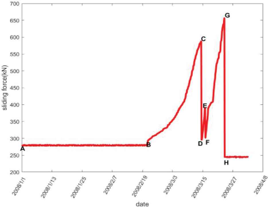
The variation trend of the sliding force at the monitoring point No.1.
3. THE BRB PREDICTION MODEL BASED ON HISTORICAL SLIDING FORCE
In the proposed model, BRB model is established to describe the nonlinear relationship between the historical/current sliding force and the future sliding force. In BRB model, the activated belief rules are fused by the evidence reasoning (ER) algorithm. Finally, the future sliding force can be calculated from the fused results. To better understand the model, the list of the variables is shown in Table 1.
| Variables | Explanation |
|---|---|
| Ai | The reference value of the i-th input variable |
| Vj | The reference value of the predicted sliding force |
| The belief degree of Vj in the k-th rule | |
| The relative importance of the k-th rule | |
| The relative importance of the input attribute |
|
| L | The number of rules |
| The number of clusters of the output vectors | |
| The number of clusters of the i-th input variable | |
| mk | The time label of the minimum distance sample vector |
| wk | The activated weight of the k-th rule |
| The matching degree of the i-th input variable and the reference value |
|
| The interval width of the reference value of the i-th input variable | |
| Reduction factor | |
| Enlargement factor | |
| Relative position ratio |
The list of variables and parameters of the belief rule-based (BRB) prediction model.
3.1. The BRB-Based Sliding Force Prediction Model
The BRB system is an extension of the traditional IF–THEN rule expert system. It is capable of modeling and inferring incomplete, fuzzy, and uncertain data. And constructing belief rules is a key part of establishing a BRB system [26]. In a belief rule, each antecedent attribute has its corresponding reference value, and each consequent attribute corresponds to a belief distribution. As shown in the Eq. (2), the k-th rule is taken as an example, where
Based on the above interpretation, the construction of the BRB sliding force prediction model and its inference process can be divided into the following steps:
Confirm the input and output variables together with their reference values Ai and Vj.
Form the antecedent attributes of total
The input variable is adopted to activate rules of the BRB, and ER algorithm is adopted to fuse the belief distribution of the consequent attributes of the activated rules, from which
In the following sections, a detailed analysis and introduction of the above steps are given.
| The BRB System | The Physical Interpretation of Variables and Parameters |
|---|---|
| Antecedent attribute | Input variable |
| Reference value set |
The reference value of the i-th input variable Ai |
| The number of reference values of antecedent attributes Li | Li is the number of parameter values of the i-th input variable |
| The antecedent of the k-th rule, |
Reference values of f(t) in the k-th rule |
| The consequent of the k-th rule |
|
| Number of conclude attributes J | J is the number of output variable parameter values |
| Rule weight |
The relative importance of the k-th rule |
| Attribute weight |
The relative importance of input attribute |
The physical interpretation of input and output variables of a belief rule-based (BRB) model.
3.2. Obtaining Input and Output Reference Values of BRB Based on Historical Data
Taking the case of monitoring point No.1 shown in Figure 3 as an example, the sliding force in Section BC is used as historical data to confirm the input and output variables together with their reference values in the BRB model, respectively. According to the variation trend of the data in Section BC, the input variables are selected as in Eq. (3).
Concretely, compared with the sliding force observations obtained in single time
To avoid the randomness and subjectivity of the initial parameters of the model caused by the reference value given by the expert experience, K-means is adopted to cluster the subsets into K groups so that the selected reference value is in line with the change of the samples, thus, a better fusion calculation can be obtained. Specifically, K-means clustering is implemented on the subsets
3.3. Constructing BRB Based on Historical Data
After the input and output reference values are confirmed, the belief rules L1×L2×…×LI are constructed to form a BRB. Then
After matching with
3.4. Obtaining Predicted Sliding Force Based on ER Algorithm
In the constructed BRB, the activated weight wk of the input variables
Here,
After the activated rule weights have been fixed, ER algorithm is adopted to fuse the belief distribution of consequent attribute with a different activated degree, so as to obtain the corresponding output of the input
Finally, the predicted sliding force
4. BRB MODEL TRANSFER AND ONLINE UPDATE STRATEGY
In this paper, the BRB sliding force prediction model at monitoring point No.1 is denoted as BRBa. It aims to use BRBa to predict sliding force on other slopes or adjacent monitoring points with similar geological conditions. As shown in Figure 2, monitoring point No.2 is adjacent to monitoring point No.1 and the BRB sliding force prediction model at monitoring point No.2 is represented as BRBb with the sliding force curve shown in Figure 4. By comparing Section BC in Figure 3 and Section
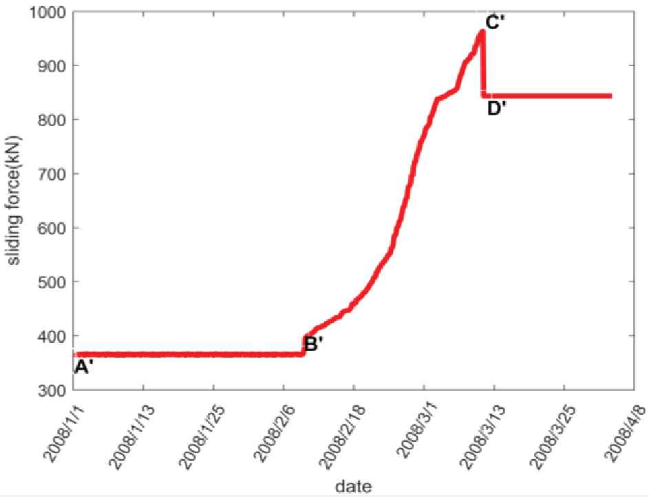
The variation trend of the sliding force at the monitoring point No.2.
4.1. Parameter Transfer of BRB Sliding Force Prediction Model for New Monitoring Point
The transferring of input and output reference values in the BRB model is actually to transplant the change law of the reference value in BRBa to BRBb. Thus, the position law of the reference value in BRBa is calculated, and then the reference values can be transferred after the abnormal variation of the sliding force at point No.2 is detected. The details are shown in the following three steps:
Step 1: Calculate the relative position ratio of the input and output reference values in BRBa.
Firstly, the interval width of the input and output reference values in BRBa can be obtained from Eq. (12), where
Secondly, the relative position ratio
Step 2: Determine the minimum and maximum of the input and output reference values in BRBb.
Specifically, the input and output of BRBb are denoted as
Step 3: Determine other input and output reference values in BRBb.
Step 1 actually describes the distribution or relationship of the input and output reference values in their respective variation ranges in BRBa. After the variation range of
4.2. SLP-based Online Optimization of Belief Parameters of the Consequent Attribute of Belief Rule
The obtained BRBb model is a relatively rough model, because
And the Q historical data samples of the monitoring point No.2 which are obtained online can be adopted to do optimization. For example, if
SLP is adopted to solve online optimization problems. To be specific, the optimal belief degrees obtained at time t will be used as the initial values of the belief degrees at time
Step 1: Calculate the first-order partial derivative of the nonlinear optimization objective function.
Based on the parameter optimization model in Eq. (17), the first-order partial derivative of the objective function
Step 2: Determine the moving limits of the optimized parameters.
The selection of moving limits directly affects the effectiveness of the SLP optimization algorithm. Specifically, large moving limits will reduce accuracy, while small moving limits lead to the increment of the number of iterations and calculation thereby extending of the program running time. Here, the upper bound of the parameters to be optimized is shown in Eq. (20). Normally, the moving limits are set less than or equal to 10% of this upper bound, which is less than or equal to 0.1.
Step 3: Use linear programming to obtain local optimal value.
A search space is established by setting the initial points and moving limits. And a linear programming method, e.g., an interior point method, is used to complete the search process [28, 29]. Specifically, if the intersection of the search space and the linearized feasible solution space is empty, the search space needs to be expanded by increasing the moving limits. If there is an intersection, the optimal solution of the linear programming problem will be searched in intersection [30]. Next, take the obtained optimal solution as a new initial point, re-linearize the original nonlinear optimization objective function, and iteratively execute the entire process until the given stopping criterion is achieved.
Step 4: Stop criterion.
When 1) the moving limits of all parameters are reduced to a significantly small value, or 2) the value of the parameters or the value of the objective function does not change significantly during two iterations, the SLP iteration process should be stopped.
5. EXPERIMENTS AND ANALYSIS OF SLIDING FORCE PREDICTION
5.1. Construct BRBa Based on Historical Data of Monitoring Point No.1
BRBa is constructed by the sliding force of the rising stage (Section BC) at the monitoring point No.1 in Figure 3. Concretely, the sampling time corresponding to B is 3 o'clock on February 22, 2008 and the sliding force increases from a relatively stable 278.5 kN to 294.08 kN at this point, where kN is an international unit for measuring the size of the force. The sampling time corresponding to C is 9 o'clock on March 15, 2008, the sliding force drops from the largest 588.95 kN to 296.02 kN at this point, which indicates that the structure of the slope body has changed at this moment. All in all, it takes 486 hours from the abnormal increase of the sliding force at B to the change of the slope body structure at C, and 178 sets of measurement data are collected.
5.1.1. Determine input and output reference values in BRBa
Regarding to the 178 sets of data, a dataset
| Input variable f1(t) | Semantic value | A1,1(VS) | A1,2(PS) | A1,3(PM) | A1,4(PL) | A1,5(ML) | A1,6(VL) |
| Reference value | 295.0855 | 320.3768 | 382.6278 | 460.0012 | 549.9463 | 585.5067 | |
| Input variable f2(t) | Semantic value | A2,1(VS) | A2,2(PS) | A2,3(PM) | A2,4(PL) | A2,5(ML) | A2,6(VL) |
| Reference value | −0.2140 | 0.7225 | 1.5206 | 3.0613 | 3.4339 | 10.4008 | |
| Input variable f3(t) | Semantic value | A3,1(VS) | A3,2(PS) | A3,3(PM) | A3,4(PL) | A3,5(ML) | A3,6(VL) |
| Reference value | 0.0000 | 0.7209 | 1.5265 | 3.0571 | 3.4091 | 6.8430 | |
| Output variable y(t+ 2) | Semantic value | V1(VS) | V2(PS) | V3(PM) | V4(PL) | V5(ML) | V6(VL) |
| Reference value | 295.8567 | 321.8439 | 385.7263 | 466.7651 | 559.0389 | 587.9533 |
The reference value (semantic value) of input and output variables in BRBa.
5.1.2. Obtain belief rules in BRBa
Based on the reference values provided in Table 3, BRBa can be constructed, and the k-th rule is expressed as Eq. (21), where
And the weight of the rule
| k | The Combination of Antecedent Reference Values | The Consequent Belief Distribution |
|||||
|---|---|---|---|---|---|---|---|
| β1 | β2 | β3 | β4 | β5 | β6 | ||
| 1 | VS |
0.9209 | 0.0791 | 0 | 0 | 0 | 0 |
| 2 | VS |
0.9407 | 0.0593 | 0 | 0 | 0 | 0 |
| 3 | VS |
0.9407 | 0.0593 | 0 | 0 | 0 | 0 |
| 4 | VS |
0.9407 | 0.0593 | 0 | 0 | 0 | 0 |
| 5 | VS |
0.9407 | 0.0593 | 0 | 0 | 0 | 0 |
| 96 | VS |
0 | 0 | 0.9724 | 0.0276 | 0 | 0 |
| 97 | VS |
0 | 0 | 0.9599 | 0.0401 | 0 | 0 |
| 98 | VS |
0 | 0.0285 | 0.9715 | 0 | 0 | 0 |
| 99 | PM |
0 | 0.0285 | 0.9715 | 0 | 0 | 0 |
| 137 | PL |
0 | 0 | 0.013 | 0.987 | 0 | 0 |
| 138 | PL |
0 | 0 | 0.013 | 0.987 | 0 | 0 |
| 139 | PL |
0 | 0 | 0 | 0.9446 | 0.0554 | 0 |
| 140 | PL |
0 | 0 | 0 | 0.9446 | 0.0554 | 0 |
| 212 | VL |
0 | 0 | 0 | 0 | 0 | 1 |
| 213 | VL |
0 | 0 | 0 | 0 | 0 | 1 |
| 214 | VL |
0 | 0 | 0 | 0 | 0.192 | 0.808 |
| 215 | VL |
0 | 0 | 0 | 0 | 0.192 | 0.808 |
| 216 | VL |
0 | 0 | 0 | 0 | 0.192 | 0.808 |
Part of rules in BRBa.
5.1.3. Obtain predicted sliding force based on ER algorithm
After the input variables
Take data samples
According to the reference value activated by each variable, there are 8 activated rules R2, R3, R8, R9, R38, R39, R44, R45. And Eq. (6) is adopted to calculate the corresponding activated weights such as
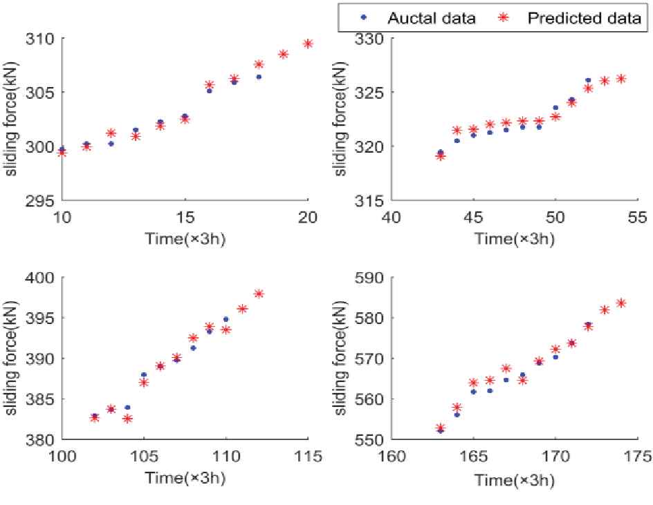
For all the remaining input variables, the corresponding predicted output values can be obtained through the above-reasoning process. As shown in Figure 5, the actual data and the predicted values at
The predicted value of sliding force in BRBa.
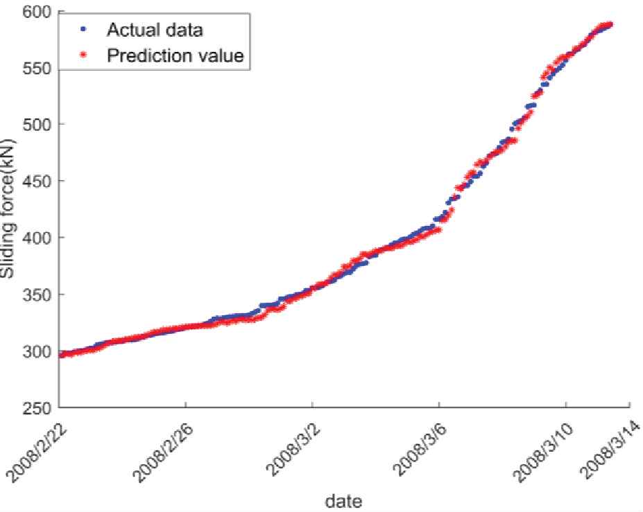
The sliding force prediction of all samples in BRBa.
5.2. Model Transfer from BRBa to BRBb
Seen from Figure 4, the sliding force at the monitoring point No.2 was observed from 0:00 on January 1, 2008, and real-time overrun detection was performed. When the increase of sliding force between two samplings exceeds 10 kN, the model transfer which is illustrated in Section 4.1 is implemented from BRBa to BRBb. For example, at sampling time B′ in Figure 4 (6:00 on February 11, 2008), the sliding force increased from 376.5 kN to 398.3655 kN, thus the change amount is over 10 kN. At this moment, the model transfer needs to be implemented.
5.2.1. Parameter transfer of BRBb model
Firstly, the interval width of the reference values in BRBa is calculated by Eq. (12). To be specific, the interval width of the input reference values is
Set the time at B′ as
| Input variable f1(t) | Semantic value | Ab1,1(VS) | Ab1,2(PS) | Ab1,3(PM) | Ab1,4(PL) | Ab1,5(ML) | Ab1,6(VL) |
| Reference value | 398.3655 | 450.5825 | 579.1081 | 738.8556 | 924.5593 | 995.9137 | |
| Input variable f2(t) | Semantic value | Ab2,1(VS) | Ab2,2(PS) | Ab2,3(PM) | Ab2,4(PL) | Ab2,5(ML) | Ab2,6(VL) |
| Reference value | −1.0410 | 1.9696 | 3.3524 | 6.0217 | 6.6673 | 17.3500 | |
| Input variable f3(t) | Semantic value | Ab3,1(VS) | Ab3,2(PS) | Ab3,3(PM) | Ab3,4(PL) | Ab3,5(ML) | Ab3,6(VL) |
| Reference value | −0.5205 | 1.6721 | 2.9590 | 5.4038 | 5.9660 | 10.4102 | |
| Output variable y(t+ 2) | Semantic value | Vb1(VS) | Vb2(PS) | Vb3(PM) | Vb4(PL) | Vb5(ML) | Vb6(VL) |
| Reference value | 398.3655 | 451.5314 | 582.2250 | 748.0180 | 930.6586 | 995.9137 |
Reference value (semantic value) of input and output variables in BRBb.
5.2.2. Online iterative optimization of belief degree parameters in BRBb based on SLP
The initial BRBb model can be generated by the parameter transfer described in Section 5.2.1. In the initial BRBb model, the number of rules and the belief distribution of the consequent attributes in each rule are consistent with BRBa as shown in Table 4, except that the reference value of antecedent attributes are replaced with BRBb as shown in Table 5. In this experiment, BRBb model makes prediction of two steps in advance
| t | |||||
|---|---|---|---|---|---|
| 3 | 399.4065 | 0.347 | 0.5205 | 402.1133 | 402.182 |
| 4 | 401.4882 | 2.0817 | 1.2143 | 404.0322 | 403.9196 |
| 5 | 402.182 | 0.6938 | 1.3877 | 403.5488 | 404.6097 |
Input variables and output variables at three moments in BRBb.
In order to increase the prediction accuracy of BRBb at subsequent times, when at
| k | The Combination of Antecedent Reference Values | The Consequent Belief Distribution |
|||||
|---|---|---|---|---|---|---|---|
| 1 | VS |
0.9209 | 0.0791 | 2.51e-15 | 8.83e-16 | 5.13e-16 | 4.26e-16 |
| 2 | VS |
0.9407 | 0.0593 | 3.26e-15 | 1.15e-15 | 6.67e-16 | 5.79e-16 |
| 7 | VS |
0.9209 | 0.0791 | 8.28e-16 | 2.91e-16 | 1.69e-16 | 1.47e-16 |
| 8 | VS |
0.9407 | 0.0593 | 1.17e-15 | 4.1e-16 | 2.37e-16 | 2.06e-16 |
| 37 | PS |
0.0044 | 0.9956 | 1.7e-14 | 1.69e-14 | 1.09e-14 | 9.79e-15 |
| 38 | PS |
0.0142 | 0.9858 | 5.0e-14 | 2.31e-14 | 1.43e-14 | 1.27e-14 |
| 43 | PS |
0.0241 | 0.9759 | 1.62e-14 | 8.38e-15 | 5.47e-15 | 4.86e-15 |
| 44 | PS |
0.0241 | 0.0759 | 2.0e-14 | 1.04e-14 | 6.81e-15 | 6.05e-15 |
The optimized rule at t = 7 in BRBbo(7).
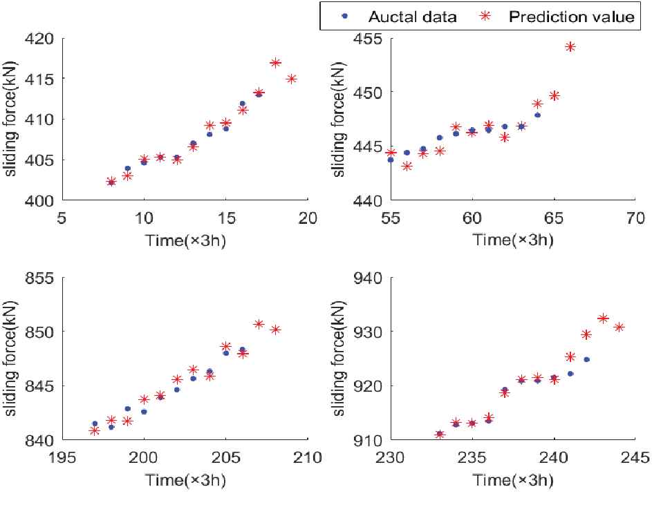
When
The sliding force prediction at part of time in BRBbo.
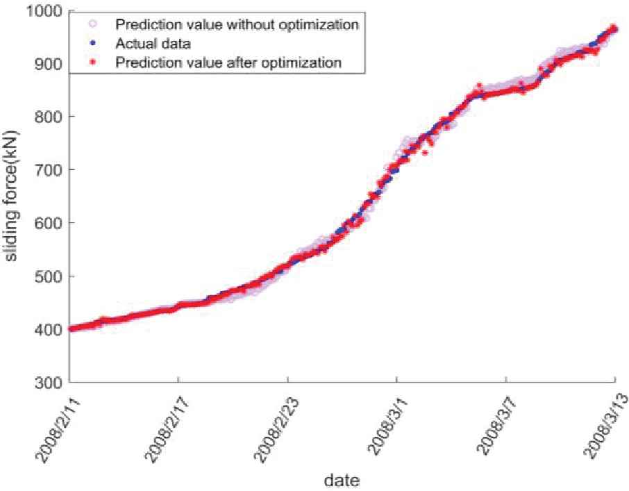
The comparison of prediction in initial BRBb and the iterative optimization BRBbo.
| k | The Combination of Antecedent Reference Values | The Consequent Belief Distribution |
|||||
|---|---|---|---|---|---|---|---|
| 1 | VS |
0.9863 | 7.29e-13 | 9.49e-13 | 1.88e-12 | 4.57e-07 | 0.0133 |
| 2 | VS |
0.9835 | 1.27e-13 | 2.83e-13 | 1.41e-12 | 1.14e-07 | 0.0165 |
| 3 | VS |
0.9455 | 0.0392 | 5.77e-10 | 1.14e-08 | 0.0076 | 0.0076 |
| 4 | VS |
0.9407 | 0.0593 | 0 | 0 | 0 | 0 |
| 5 | VS |
0.9407 | 0.0593 | 0 | 0 | 0 | 0 |
| 96 | VS |
0.0365 | 0.0108 | 0.861 | 0.0306 | 0.0306 | 0.0306 |
| 97 | VS |
0 | 0 | 0.9599 | 0.0401 | 0 | 0 |
| 98 | VS |
0 | 0.0285 | 0.9715 | 0 | 0 | 0 |
| 99 | PM |
0.0685 | 0.0277 | 0.837 | 0.0223 | 0.0223 | 0.0223 |
| 134 | PL |
0 | 0 | 0.013 | 0.987 | 0 | 0 |
| 135 | PL |
0.0487 | 0.0196 | 0.0136 | 0.9008 | 0.0086 | 0.0086 |
| 136 | PL |
0.0264 | 0.0264 | 0.0191 | 0.8577 | 0.0423 | 0.0282 |
| 137 | PL |
0.0112 | 0.0112 | 0.0112 | 0.8316 | 0.0781 | 0.0567 |
| 212 | VL |
0 | 0 | 0 | 0 | 0 | 1 |
| 213 | VL |
0 | 0 | 0 | 0 | 0 | 1 |
| 214 | VL |
0.0017 | 0.0017 | 9.52e-10 | 2.91e-11 | 0.1403 | 0.8563 |
| 215 | VL |
0.0017 | 0.0017 | 1.36e-10 | 8.02e-12 | 0.0953 | 0.9012 |
| 216 | VL |
0.0051 | 0.0051 | 7.96e-10 | 2.68e-08 | 0.1369 | 0.8529 |
The optimized belief rule base.
5.3. Expansion Test Experiment and Analysis
In order to verify the effectiveness of the proposed model transfer and parameter online optimization methods, linear disturbances and sinusoidal function disturbances are implemented on the sliding force data at monitoring point No.2, which changes the overall or local variation trends of the sliding force. As shown in the Figure 9, the upper picture shows the case of adding linear disturbance which increases the sliding force changing rate and expands the sliding force range. And the under picture demonstrates the situation of adding nonlinear disturbance which makes the local trend of the sliding force more uncertain. Model transfer and parameter optimization are implemented based on BRBa so that a new BRB is generated for sliding force prediction. The simulation results in Figure 9 prove that the proposed method has good robustness, and relatively accurate prediction results are given in both cases.
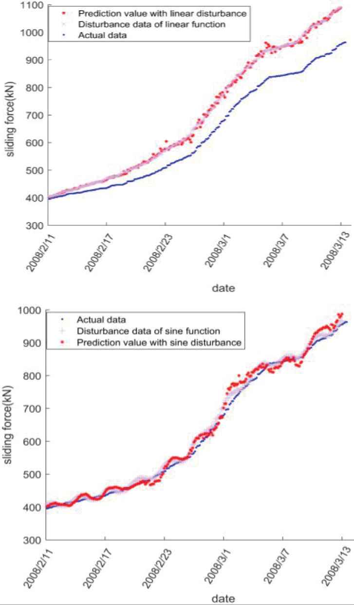
The predictions of adding different disturbances to the sliding force at monitoring point No.2.
6. SUMMARY
To tackle the uncertain problem which is caused by variation of sliding force, a method of slope sliding force prediction based on BRB inferential methodology is proposed in the paper to achieve accurate prediction of different slope sliding force measurement points. The main contributions of this paper are demonstrated as follows:
BRB prediction model based on historical data is established. A BRB prediction model is constructed so as to describe the nonlinear mapping relationship between input (history, current sliding force) and output (future sliding force). ER algorithm is adopted to fuse the belief rules which are activated by input. Based on the fused results, the prediction of the sliding force can be calculated.
A parameter transfer of the BRB sliding force prediction model for new monitoring points is proposed. Based on historical data, the BRB and the relative position ratio of the input and output reference values are determined. By transference and transformation of the determined values, the BRB and the input and output reference values of the sliding force prediction model at new monitoring points can be obtained.
Local iteration optimization of model parameters strategy is adopted. For the adaptive adjustment of BRB models at different monitoring points, SLP is used to iteratively optimize and update the parameters activated in the BRB model after transference, so as to improve the prediction accuracy of the model.
In addition, there are still some worthy problems for further discussion and research:
As the factors which influencing the slope stability are complicated, such as groundwater, fracture, ground stress, and directly obtaining the data by NPR anchor cable has some limitations, the prediction and stability analysis of slope sliding with a variety of uncertain information needs further study.
In this paper, the measurement samples of the NPR anchor cable are complete. However, the measurement data is incomplete in reality. In future studies, it is worth further discussing and extending this aspect.
When the sliding force is abrupt, the internal structure of the slope changes, and the prediction model cannot be used. How to solve the abrupt sliding force prediction needs further study.
CONFLICTS OF INTEREST
We confirm that the manuscript has been read and approved by all named authors and that there are no other persons who satisfied the criteria for authorship but are not listed. We further confirm that the order of authors listed in the manuscript has been approved by all of us.
AUTHORS' CONTRIBUTIONS
Jing Feng: conceived of the presented idea and wrote the manuscript. Xiaobin Xu: developed the theory. Pan Liu: carried out the experiment. Feng Ma: performed the calculations. Chengrong Ma: contributed to the interpretation of the results. Zhigang Tao: contributed to data preparation and analysis. All authors provided critical feedback and helped shape the research, analysis and manuscript.
ACKNOWLEDGMENTS
This work was supported by the Zhejiang Province Key R&D projects (No.2019C03104), the NSFC-Zhejiang Joint Fund for the Integration of Industrialization and Informatization (No. U1709215), the Zhejiang Provincial Basic Public Welfare Research Project (No. LGF21F020013), the Open Research Project of the State Key Laboratory of Industrial Control Technology, Zhejiang University, China (No. ICT20028), the Second Tibetan Plateau Scientific Expedition and Research Program (No. 2019QZKK0707), the NSFC (No. 61751304).
REFERENCES
Cite this article
TY  - JOUR
AU  - Jing Feng
AU  - Xiaobin Xu
AU  - Pan Liu
AU  - Feng Ma
AU  - Chengrong Ma
AU  - Zhigang Tao
PY  - 2021
DA  - 2021/02/25
TI  - Slope Sliding Force Prediction via Belief Rule-Based Inferential Methodology
JO  - International Journal of Computational Intelligence Systems
SP  - 965
EP  - 977
VL  - 14
IS  - 1
SN  - 1875-6883
UR  - https://doi.org/10.2991/ijcis.d.210216.001
DO  - 10.2991/ijcis.d.210216.001
ID  - Feng2021
ER  -