
Ameliorated Ensemble Strategy-Based Evolutionary Algorithm with Dynamic Resources Allocations
 , Syed Nouman Ali Shah1, Samir Brahim Belhaouari2, , Abdelouahed Hamdi3, *
- DOI
- 10.2991/ijcis.d.201215.005How to use a DOI?
- Keywords
- Global optimization; Soft computing; Evolutionary computing; Evolutionary algorithms (EAs); Ensemble strategy-based EAs
- Abstract
In the last two decades, evolutionary computing has become the mainstream to attract the attention of the experts in both academia and industrial applications due to the advent of the fast computer with multi-core GHz processors have had a capacity of processing over
- Copyright
- © 2021 The Authors. Published by Atlantis Press B.V.
- Open Access
- This is an open access article distributed under the CC BY-NC 4.0 license (http://creativecommons.org/licenses/by-nc/4.0/).
1. INTRODUCTION
Optimization is the mathematical process of finding either maximum or minimum value of a function in a domain of definition, subject to various constraints on the variable values. A local minimum of a function is a point where the function value is smaller than or equal to the value at nearby points. A global minimum is a point where the function value is smaller than or equal to the value at all other feasible points. Optimization problems can be classified as linear, quadratic, polynomial, nonlinear depending upon the nature of the objective functions and the constraints. Many real-world problems are naturally modeled as global optimization problems [1–8]. A general optimization problem can be modeled as follows:
Since its inception in the late 1950s, evolutionary computing methods have received significant attention due to large domain applications [19–25]. Until the present, evolutionary algorithms (EAs) under the umbrella of (evolutionary computation [EC]) have successfully and effectively tackled various test suites of benchmark functions and many real-world problems with a nonlinear, multi-modal, scalable objective, and constrained functions with complicated structures. Despite having the vast popularity of various nature-inspired and swarm-inspired EAs, still, we need to address their existing shortcomings to make them more advanced and effective by following the basic principles of rules of population evolution, procedures of self-organization and self-adaptation [26]. In general, nature-inspired-based algorithms can be categorized into EAs and swarm intelligence-based algorithms as shown in Figure 1. The EAs including the genetic algorithm (GA) [20,25,27,28], genetic programming (GP) [29], evolutionary strategies (ESs) [30,31], evolutionary programming (EP) [32] are classified as classical paradigms of EC and differential evolution (DE) [33–36] and particle swam optimization (PSO) [37,38], ant colony optimization [39,40], artificial bee colony (ABC) [41,42], cuckoo search (CS) [43], bat algorithm (BA) [44–46], Bee algorithm [47,48], and firefly algorithm (FA) [49] are new emerging population-based algorithms [50]. Despite many key features of the aforementioned EAs, they demand maximum function evaluations and spent huge computation time to solve optimization problems with complicated search space.
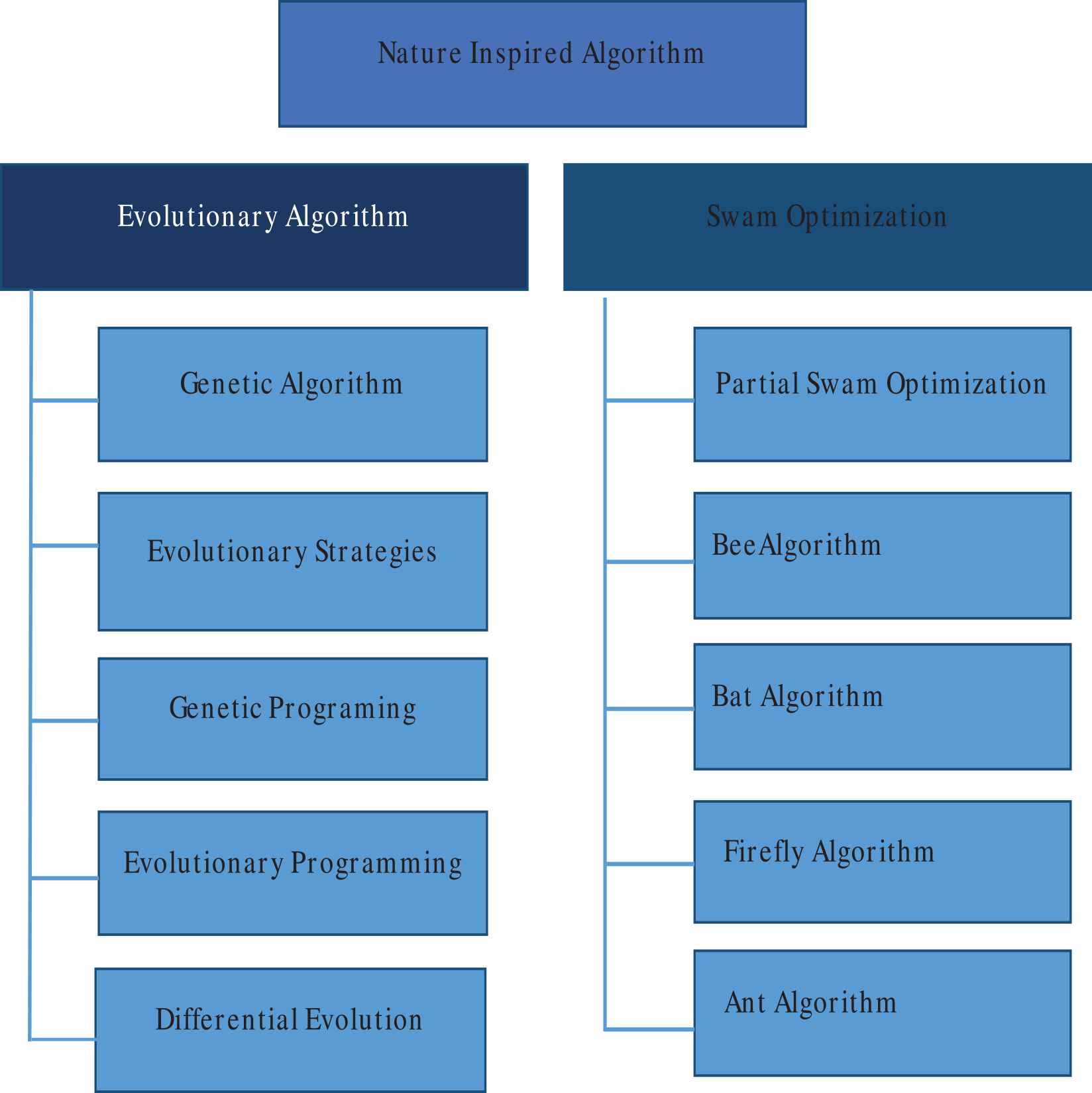
Flow chart for the classification of the nature-inspired algorithm.
However, it is still difficult and even impossible for a single EA in the existing literature of EC that always performs better on all types of benchmark functions and real-world problems [20,51,52]. In the last several years, the ensemble that multiple search operators have shown significant contribution in solving multi-objective optimization problems with the complicated shape of Pareto front (PF) and large-scale global optimization problems [3,23,53–62]. Inspired from the aforementioned algorithms, this paper also proposes an ensemble strategy-based EA with dynamic resources allocation to handle benchmark functions that are designed recently for the special session of
The rest of the paper is organized as follows: Section 2 introduces the framework of the proposed ameliorated ensemble strategy-based EA with dynamic resources allocations. Section 3 demonstrates the experimental results and characteristics of the used benchmark functions. In Section 4, we conclude our work.
2. AMELIORATED ENSEMBLE STRATEGY-BASED EA WITH DYNAMIC RESOURCES ALLOCATIONS FOR LARGE-SCALE OPTIMIZATION PROBLEMS
In the recent past two decades, several evolutionary computing methods were developed [8,19,20,61,62,69,70]. They are employing various search operators and strategies for population evolution likewise one-point, two-points, uniform crossover operators [71], trigonometric mutation [72] tournament, ranking, stochastic uniform sampling selection methods, crowding [73], sharing-based niching approaches, adaptive penalty, epsilon superiority of feasible over infeasible solutions, and ensemble constraint handling methods [70,74]. The aforementioned approaches can employ in an ensemble manner the framework of any EAs for performing numerous simulations with the main purpose to approximate the best optimal solution [35]. However, the best achievement of each approach might be associated with the fine-tuning of their corresponding control parameters either statically or additively. Furthermore, the use of different strategies and different parameters might be more appropriate at different stages of evolution and exploration of search spaces. The best setup of various paraments in the EAs can be settled based on trial and error strategies. Recently, ensemble strategies-based EAs have gained much popularity in order to utilize the key features of a diverse set of approaches in the existing literature of evolutionary computing [57,58,62,74–76]. In this paper, we have proposed an ensemble strategy-based EA for solving diverse nature of benchmark functions that are recently designed for the special session of IEEE-CEC'17 [63]. The framework of the suggested ameliorated algorithm is hereby explained in the Algorithm 1. The suggested algorithm denoted by ESEA1 engages the most popular existing EAs, namely, PSO [37,38,64], DE [36], BA [45] and TLBO [65–68] to perform their search process. The proposed algorithm allocates resources to their constituent algorithms dynamically following the steps from 34 to 38 of the Algorithm 1. As can see in steps 4 to step 5 of Algorithm 1, the constituent algorithms have allocated the same resources. Further, the formula in step 36 of the Algorithm 1 is used to allocate the resources dynamically.
Algorithm 1: The Framework of the Ameliorated Ensemble Strategy-Based Evolutionary Algorithm
1:
2: Evaluate function values of
3: Initially, divide the population set of size
4:
5:
6: for
7: if
8:
9:
10: end if
11: if
12:
13: end if
14: if
15:
16:
17:
18:
19:
20: end if
21: if
22: Generate a random
23: end if
24: if
25: Update learner
26: end if
27: Compute the objective function values of new set of population.
28: if
29:
30: else
31:
32: end if
33: Compute the success rate
34: for
35:
36: Update the set of sub-population by using formula:
37: end for
38:
39: end for
In the proposed algorithm, TLBO has been used as a constituent algorithm that employs a group of learners whose fitness level is evaluated upon their results or grades. The grade of each learner is then updated based on their learning attained from the teacher and their interaction with other learners. Two phases are involved in TLBO operation including the teacher phase and learner phase. The learning enthusiasm values of learners as described in [77] as given under:
The polynomial mutation is described as under:
Algorithm 2: The Framework of the Particle Swarm Optimization
1:
2: Compute the objective function values,
3:
4: while
5:
6:
7: Compute the objective function values of new population set of solutions,
8: if
9:
10: else
11:
12: end if
13:
14: end while
2.1. Differential Evolution
DE is one of the most popular EAs that was first proposed by Rainer Storn and Kenneth Price for solving the Chebychev polynomial fitting problems [36]. DE uses the idea difference to perturb their population. DE is similar to other existing generates its population uniformly and randomly. Then, it applies the fundamental evolutionary operators include “mutation, crossover, and selection” to perform its search process in the whole course of the optimization process. The parameters involved in the framework DE including N (population size),
In DE [35,36,84],
DE/rand/1:
DE/best/1:
DE/rand-to-best/1:
DE/current-to-best/1:
where
2.1.1. Crossover operation
A crossover is a procedure to exchange information among the previous and current population to produce a new population. It is normally applied for the exploration of different valuable regions of search space aiming at to maintain diversity among the population for further evolution. In DE, the crossover operator applied on each
2.1.2. Selection operation
The selection operation is conducted among parent solutions
2.2. Particle Swam Optimization
PSO algorithm was first proposed by James Kennedy and Russell Eberhart [38]. PSO was mainly inspired by the social behaviors and interaction of swarm as encountered in nature likewise animal herds, bird flocking, and schooling of fish. It uses a swarm of insects while performing the search process and each member of the group is called particle [86]. Due to its simple search mechanism, computational efficiency, and easy implementation, PSO has successfully tackled many optimization problems. Each Particle of PSO utilizes their personal best experience and the global experience of their neighbors to adaptively adjust its velocity
where
3. BENCHMARK FUNCTIONS AND EXPERIMENTAL RESULTS
In this research work, we assess the performance of the proposed ameliorated ensemble strategy-based EA with dynamic resources allocations by using
| No | Objective Function | Optimal Solution | |
|---|---|---|---|
| UF | 1 | Shifted and Rotated Bent Cigar Function | 100 |
| 2 | Shifted and Rotated Sum of Different Power Function* | 200 | |
| 3 | Shifted and Rotated Zakharov Function | 300 | |
| SMF | 4 | Shifted and Rotated Rosenbrocks Function | 400 |
| 5 | Shifted and Rotated Rastrigins Function | 500 | |
| 6 | Shifted and Rotated Expanded Scaffers F6 Function | 600 | |
| 7 | Shifted and Rotated Lunacek BiRastrigin Function | 700 | |
| 8 | Shifted and Rotated Non-Continuous Rastrigins Function | 800 | |
| 9 | Shifted and Rotated Levy Function | 900 | |
| 10 | Shifted and Rotated Schwefels Function | 1000 | |
| HF | 11 | Hybrid Function 1 (N = 3) | 1100 |
| 12 | Hybrid Function 2 (N = 3) | 1200 | |
| 13 | Hybrid Function 3 (N = 3) | 1300 | |
| 14 | Hybrid Function 4 (N = 4) | 1400 | |
| 15 | Hybrid Function 5 (N = 4) | 1500 | |
| 16 | Hybrid Function 6 (N = 4) | 1600 | |
| 17 | Hybrid Function 6 (N = 5) | 1700 | |
| 18 | Hybrid Function 6 (N = 5) | 1800 | |
| 19 | Hybrid Function 6 (N = 5) | 1900 | |
| 20 | Hybrid Function 6 (N = 6) | 2000 | |
| CF | 21 | Composition Function 1 (N = 3) | 2100 |
| 22 | Composition Function 2 (N= 3) | 2200 | |
| 23 | Composition Function 3 (N = 4) | 2300 | |
| 24 | Composition Function 4 (N = 4) | 2400 | |
| 25 | Composition Function 5 (N = 5) | 2500 | |
| 26 | Composition Function 6 (N = 5) | 2600 | |
| 27 | Composition Function 7 (N = 6) | 2700 | |
| 28 | Composition Function 8 (N = 6) | 2800 | |
| 29 | Composition Function 9 (N = 3) | 2900 | |
| 30 | Composition Function 10 (N = 3) | 3000 |
Features of the 2017 IEEE congress on evolutionary computing (IEEE-CEC'17) benchmark functions.
3.1. Computing Platform and Experimental Settings
All experiments were performed on a computer with Intel Core
3.2. Parameters Settings
In our carried out experiment, we have settled different parameters as the lower bound
3.3. Characteristics of Benchmark Functions and Discussion Over Experimental Results
Benchmark functions might determine strict rules on the termination conditions to execute the suggested algorithm and establish a fair comparison against some existing algorithms. The same budget of function evaluations,
In Table 1,
Tables 2 and 3 clearly exhibit that the proposed ESEA algorithm has performed much better than PSO and DE, and it has tackled each benchmark functions more effectively, especially,
| Problem No | Optimum | Algorithm | Best | Worst | Mean | St. Dev. | CPU Time/Run(s) |
|---|---|---|---|---|---|---|---|
| DE | |||||||
| F01 | PSO | ||||||
| ESEA | |||||||
| DE | |||||||
| F02 | PSO | ||||||
| ESEA | |||||||
| DE | |||||||
| F03 | PSO | ||||||
| ESEA | |||||||
| DE | |||||||
| F04 | PSO | ||||||
| ESEA | |||||||
| DE | |||||||
| F05 | PSO | ||||||
| ESEA | |||||||
| DE | |||||||
| F06 | PSO | ||||||
| ESEA | |||||||
| DE | |||||||
| F07 | PSO | ||||||
| ESEA | |||||||
| DE | |||||||
| F08 | PSO | ||||||
| ESEA | |||||||
| DE | |||||||
| F09 | PSO | ||||||
| ESEA | |||||||
| DE | |||||||
| F10 | PSO | ||||||
| ESEA | |||||||
| DE | |||||||
| F11 | PSO | ||||||
| ESEA | |||||||
| DE | |||||||
| F12 | PSO | ||||||
| ESEA | |||||||
| DE | |||||||
| F13 | PSO | ||||||
| ESEA | |||||||
| DE | |||||||
| F14 | PSO | ||||||
| ESEA | |||||||
| DE | |||||||
| F15 | PSO | ||||||
| ESEA |
PSO, particle swarm optimization; DE, differential eveloution; CEC, congress on evolutionary computing.
Numerical results supplied by our proposed ESEA versus DE and PSO by solving
| Problem No | Optimum | Algorithm | Best | Worst | Mean | St. Dev. | CPU Time/Run(s) |
|---|---|---|---|---|---|---|---|
| F16 | PSO | ||||||
| ESEA | |||||||
| DE | |||||||
| F17 | PSO | ||||||
| ESEA | |||||||
| DE | |||||||
| F18 | PSO | ||||||
| ESEA | |||||||
| DE | |||||||
| F19 | PSO | ||||||
| ESEA | |||||||
| DE | |||||||
| F20 | PSO | ||||||
| ESEA | |||||||
| DE | |||||||
| F21 | PSO | ||||||
| ESEA | |||||||
| DE | |||||||
| F22 | PSO | ||||||
| ESEA | |||||||
| DE | |||||||
| F23 | PSO | ||||||
| ESEA | |||||||
| DE | |||||||
| F24 | PSO | ||||||
| ESEA | |||||||
| DE | |||||||
| F25 | PSO | ||||||
| ESEA | |||||||
| DE | |||||||
| F26 | PSO | ||||||
| ESEA | |||||||
| DE | |||||||
| F27 | PSO | ||||||
| ESEA | |||||||
| DE | |||||||
| F28 | PSO | ||||||
| ESEA | |||||||
| DE | |||||||
| F29 | PSO | ||||||
| ESEA |
PSO, particle swarm optimization; DE, differential eveloution; CEC, congress on evolutionary computing.
Numerical results furnished by our proposed ESEA versus DE and PSO by solving
Tables 4 and 5 summarizes the numerical results incurred by our proposed ESEA algorithm while solving each benchmark function of the IEEE-CEC'17 test suite [63] with thirty decision variables. The first column of Tables 4 and 5 present the best objective function values approximated by ESEA algorithm in comparison with PSO and DE Algorithm with the same parameter settings and resources allocations. The benchmark functions used in our carried out experiments, namely,
| Problem No | Optimum | Algorithm | Best | Worst | Mean | St. Dev. | CPU Time/Run(s) |
|---|---|---|---|---|---|---|---|
| DE | |||||||
| F01 | PSO | ||||||
| ESEA | |||||||
| DE | |||||||
| F02 | PSO | ||||||
| ESEA | |||||||
| DE | |||||||
| F03 | PSO | ||||||
| ESEA | |||||||
| DE | |||||||
| F04 | PSO | ||||||
| ESEA | |||||||
| DE | |||||||
| F05 | PSO | ||||||
| ESEA | |||||||
| DE | |||||||
| F06 | PSO | ||||||
| ESEA | |||||||
| DE | |||||||
| F07 | PSO | ||||||
| ESEA | |||||||
| DE | |||||||
| F08 | PSO | ||||||
| ESEA | |||||||
| DE | |||||||
| F09 | PSO | ||||||
| ESEA | |||||||
| DE | |||||||
| F10 | PSO | ||||||
| ESEA | |||||||
| DE | |||||||
| F11 | PSO | ||||||
| ESEA | |||||||
| DE | |||||||
| F12 | PSO | ||||||
| ESEA | |||||||
| DE | |||||||
| F13 | PSO | ||||||
| ESEA | |||||||
| DE | |||||||
| F14 | PSO | ||||||
| ESEA | |||||||
| DE | |||||||
| F15 | PSO | ||||||
| ESEA |
PSO, particle swarm optimization; DE, differential eveloution; CEC, congress on evolutionary computing.
Numerical results provided by our proposed ESEA versus DE and PSO by solving
| Problem No | Optimum | Algorithm | Best | Worst | Mean | St. Dev. | CPU Time/Run(s) |
|---|---|---|---|---|---|---|---|
| DE | |||||||
| F16 | PSO | ||||||
| ESEA | |||||||
| DE | |||||||
| F17 | PSO | ||||||
| ESEA | |||||||
| DE | |||||||
| F18 | PSO | ||||||
| ESEA | |||||||
| DE | |||||||
| F19 | PSO | ||||||
| ESEA | |||||||
| DE | |||||||
| F20 | PSO | ||||||
| ESEA | |||||||
| DE | |||||||
| F21 | PSO | ||||||
| ESEA | |||||||
| DE | |||||||
| F22 | PSO | ||||||
| ESEA | |||||||
| DE | |||||||
| F23 | PSO | ||||||
| ESEA | |||||||
| DE | |||||||
| F24 | PSO | ||||||
| ESEA | |||||||
| DE | |||||||
| F25 | PSO | ||||||
| ESEA | |||||||
| DE | |||||||
| F26 | PSO | ||||||
| ESEA | |||||||
| DE | |||||||
| F27 | PSO | ||||||
| ESEA | |||||||
| DE | |||||||
| F28 | PSO | ||||||
| ESEA | |||||||
| DE | |||||||
| F29 | PSO | ||||||
| ESEA |
PSO, particle swarm optimization; DE, differential eveloution; CEC, congress on evolutionary computing.
Numerical results gathered by our proposed ESEA versus DE and PSO by solving
Tables 6 and 7 offer the numerical results accumulated by the proposed ESEA algorithm in terms of the minimum function values, average function values, standard deviation values, and maximum function values by solving each benchmark functions with fifty decision variables [63]. ESEA has efficiently tackled almost all test problems, especially,
| Problem No | Optimum | Algorithm | Best | Worst | Mean | St. Dev. | CPU Time/Run(s) |
|---|---|---|---|---|---|---|---|
| DE | |||||||
| F01 | PSO | ||||||
| ESEA | |||||||
| DE | |||||||
| F02 | PSO | ||||||
| ESEA | |||||||
| DE | |||||||
| F03 | PSO | ||||||
| ESEA | |||||||
| DE | |||||||
| F04 | PSO | ||||||
| ESEA | |||||||
| DE | |||||||
| F05 | PSO | ||||||
| ESEA | |||||||
| DE | |||||||
| F06 | PSO | ||||||
| ESEA | |||||||
| DE | |||||||
| F07 | PSO | ||||||
| ESEA | |||||||
| DE | |||||||
| F08 | PSO | ||||||
| ESEA | |||||||
| DE | |||||||
| F09 | PSO | ||||||
| ESEA | |||||||
| DE | |||||||
| F10 | PSO | ||||||
| ESEA | |||||||
| DE | |||||||
| F11 | PSO | ||||||
| ESEA | |||||||
| DE | |||||||
| F12 | PSO | ||||||
| ESEA | |||||||
| DE | |||||||
| F13 | PSO | ||||||
| ESEA | |||||||
| DE | |||||||
| F14 | PSO | ||||||
| ESEA | |||||||
| DE | |||||||
| F15 | PSO | ||||||
| ESEA |
PSO, particle swarm optimization; DE, differential eveloution; CEC, congress on evolutionary computing.
Numerical results accumulated by our proposed ESEA versus DE and PSO by solving
| Problem No | Optimum | Algorithm | Best | Worst | Mean | St. Dev. | CPU Time/Run(s) |
|---|---|---|---|---|---|---|---|
| DE | |||||||
| F16 | PSO | ||||||
| ESEA | |||||||
| DE | |||||||
| F17 | PSO | ||||||
| ESEA | |||||||
| DE | |||||||
| F18 | PSO | ||||||
| ESEA | |||||||
| DE | |||||||
| F19 | PSO | ||||||
| ESEA | |||||||
| DE | |||||||
| F20 | PSO | ||||||
| ESEA | |||||||
| DE | |||||||
| F21 | PSO | ||||||
| ESEA | |||||||
| DE | |||||||
| F22 | PSO | ||||||
| ESEA | |||||||
| DE | |||||||
| F23 | PSO | ||||||
| ESEA | |||||||
| DE | |||||||
| F24 | PSO | ||||||
| ESEA | |||||||
| DE | |||||||
| F25 | PSO | ||||||
| ESEA | |||||||
| DE | |||||||
| F26 | PSO | ||||||
| ESEA | |||||||
| DE | |||||||
| F27 | PSO | ||||||
| ESEA | |||||||
| DE | |||||||
| F28 | PSO | ||||||
| ESEA | |||||||
| DE | |||||||
| F29 | PSO | ||||||
| ESEA |
PSO, particle swarm optimization; DE, differential eveloution; CEC, congress on evolutionary computing.
Numerical results accumulated by our proposed ESEA versus DE and PSO by solving
Tables 8 and 9 provides the numerical results of the proposed algorithm versus GA by solving each benchmark function in ten dimensions. Tables 10 and 11 includes the numerical results of each benchmark function with thirty decision variables. The numerical results obtained by proposed ESEA versus GA by solving
| Problem No | Optimum | Algorithm | Best | Worst | Mean | St. Dev. | CPU Time/Run(s) |
|---|---|---|---|---|---|---|---|
| F01 | GA | ||||||
| ESEA-II | |||||||
| F02 | GA | ||||||
| ESEA-II | |||||||
| F03 | GA | ||||||
| ESEA-II | |||||||
| F04 | GA | ||||||
| ESEA-II | |||||||
| F05 | GA | ||||||
| ESEA-II | |||||||
| F06 | GA | ||||||
| ESEA-II | |||||||
| F07 | GA | ||||||
| ESEA-II | |||||||
| F08 | GA | ||||||
| ESEA-II | |||||||
| F09 | GA | ||||||
| ESEA-II | |||||||
| F10 | GA | ||||||
| ESEA-II | |||||||
| F11 | GA | ||||||
| ESEA-II | |||||||
| F12 | GA | ||||||
| ESEA-II | |||||||
| F13 | GA | ||||||
| ESEA-II | |||||||
| F14 | GA | ||||||
| ESEA-II | |||||||
| F15 | GA | ||||||
| ESEA-II |
PSO, particle swarm optimization; GA, genetic algorithm; CEC, congress on evolutionary computing.
Numerical results provided by our proposed ESEA versus GA by solving
| Problem No | Optimum | Algorithm | Best | Worst | Mean | St. Dev. | CPU Time/Run(s) |
|---|---|---|---|---|---|---|---|
| F16 | GA | ||||||
| ESEA-II | |||||||
| F17 | GA | ||||||
| ESEA-II | |||||||
| F18 | GA | ||||||
| ESEA-II | |||||||
| F19 | GA | ||||||
| ESEA-II | |||||||
| F20 | GA | ||||||
| ESEA-II | |||||||
| F21 | GA | ||||||
| ESEA-II | |||||||
| F22 | GA | ||||||
| ESEA-II | |||||||
| F23 | GA | ||||||
| ESEA-II | |||||||
| F24 | GA | ||||||
| ESEA-II | |||||||
| F25 | GA | ||||||
| ESEA-II | |||||||
| F26 | GA | ||||||
| ESEA-II | |||||||
| F27 | GA | ||||||
| ESEA-II | |||||||
| F28 | GA | ||||||
| ESEA-II | |||||||
| F29 | GA | ||||||
| ESEA-II |
PSO, particle swarm optimization; GA, genetic algorithm; CEC, congress on evolutionary computing.
Numerical results provided by our proposed ESEA versus GA by solving
| Problem No | Optimum | Algorithm | Best | Worst | Mean | St. Dev. | CPU Time/Run(s) |
|---|---|---|---|---|---|---|---|
| F01 | GA | ||||||
| ESEA-II | |||||||
| F02 | GA | ||||||
| ESEA-II | |||||||
| F03 | GA | ||||||
| ESEA-II | |||||||
| F04 | GA | ||||||
| ESEA-II | |||||||
| F05 | GA | ||||||
| ESEA-II | |||||||
| F06 | GA | ||||||
| ESEA-II | |||||||
| F07 | GA | ||||||
| ESEA-II | |||||||
| F08 | GA | ||||||
| ESEA-II | |||||||
| F09 | GA | ||||||
| ESEA-II | |||||||
| F10 | GA | ||||||
| ESEA-II | |||||||
| F11 | GA | ||||||
| ESEA-II | |||||||
| F12 | GA | ||||||
| ESEA-II | |||||||
| F13 | GA | ||||||
| ESEA-II | |||||||
| F14 | GA | ||||||
| ESEA-II | |||||||
| F15 | GA | ||||||
| ESEA-II |
PSO, particle swarm optimization; GA, genetic algorithm; CEC, congress on evolutionary computing.
Numerical results provided by our proposed ESEA versus GA by solving
| Problem No | Optimum | Algorithm | Best | Worst | Mean | St. Dev. | CPU Time/Run(s) |
|---|---|---|---|---|---|---|---|
| F16 | GA | ||||||
| ESEA-II | |||||||
| F17 | GA | ||||||
| ESEA-II | |||||||
| F18 | GA | ||||||
| ESEA-II | |||||||
| F19 | GA | ||||||
| ESEA-II | |||||||
| F20 | GA | ||||||
| ESEA-II | |||||||
| F21 | GA | ||||||
| ESEA-II | |||||||
| F22 | GA | ||||||
| ESEA-II | |||||||
| F23 | GA | ||||||
| ESEA-II | |||||||
| F24 | GA | ||||||
| ESEA-II | |||||||
| F25 | GA | ||||||
| ESEA-II | |||||||
| F26 | GA | ||||||
| ESEA-II | |||||||
| F27 | GA | ||||||
| ESEA-II | |||||||
| F28 | GA | ||||||
| ESEA-II | |||||||
| F29 | GA | ||||||
| ESEA-II |
PSO, particle swarm optimization; GA, genetic algorithm; CEC, congress on evolutionary computing.
Numerical results provided by our proposed ESEA versus GA by solving
The second column of the Tables 8–13 include the known optimal solution of each used benchmark function denoted by
Figure 2 displays the evolution in minimum objective function values concerning ESEA, PSO, and DE algorithm for benchmark function,
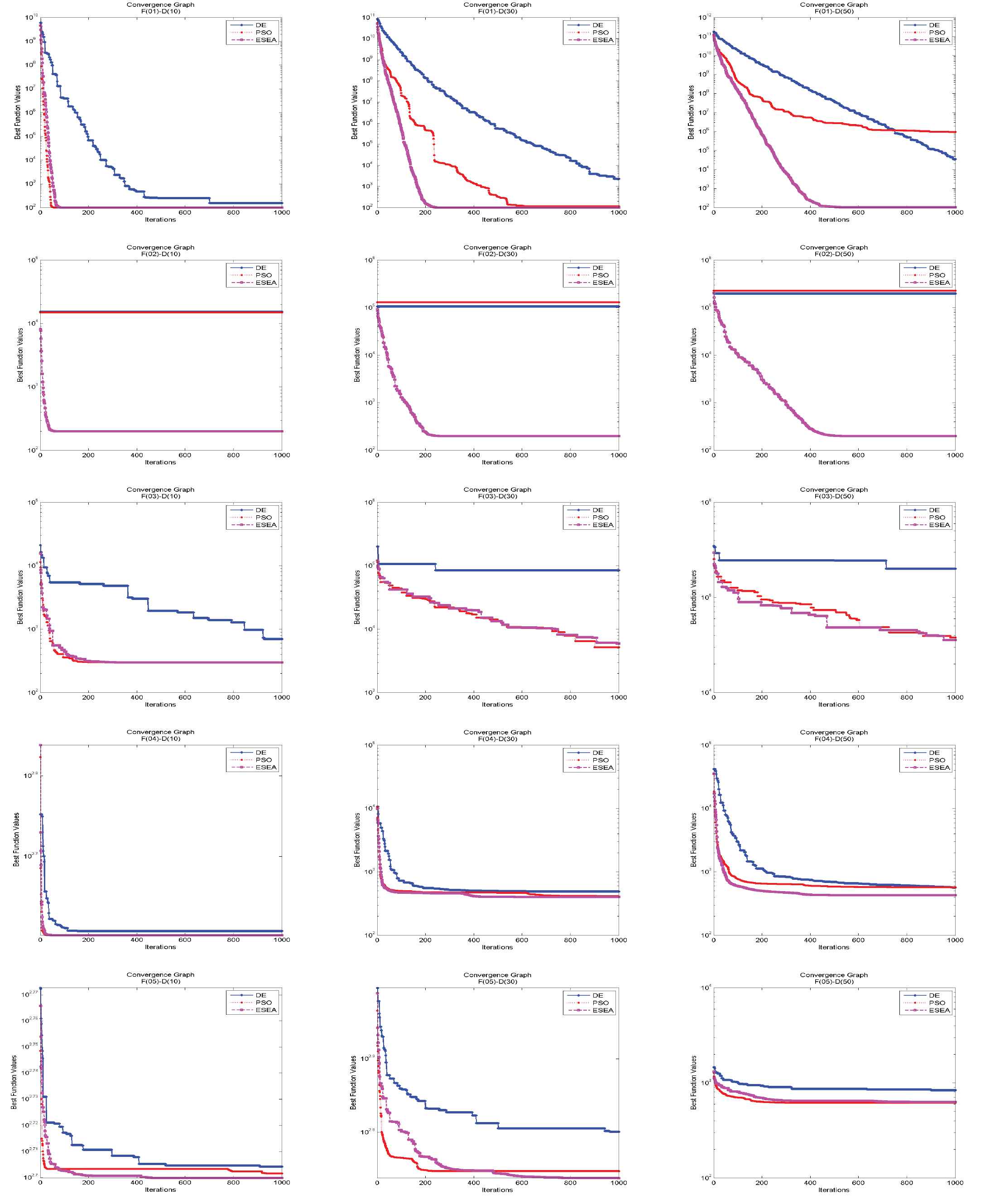
Evolution in the best function values of panel is for problems with fifty dimension.
Figure 3 demonstrates the convergence graph of the ESEA, PSO, and DE algorithm by solving the benchmark functions from
Evolution in the best function values of panel is for problems with fifty dimension.
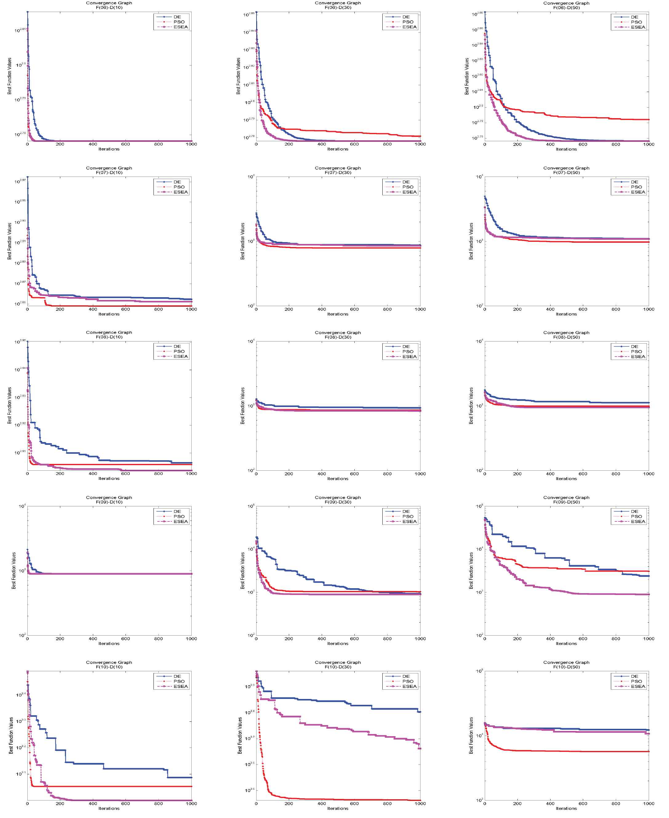
The evolutions in the minimum objective function values, when applying ESEA, PSO, and DE algorithms over benchmark function,
Evolution in the best function values of panel is for problems with fifty dimension.
The convergence graphs displayed by ESEA, PSO, and DE algorithm by solving benchmark functions likewise

Evolution in the best function values of panel is for problems with fifty dimension.
The convergence speed toward the known optimal value of the benchmark functions denoted by

Evolution in the best function values of panel is for problems with fifty dimension.
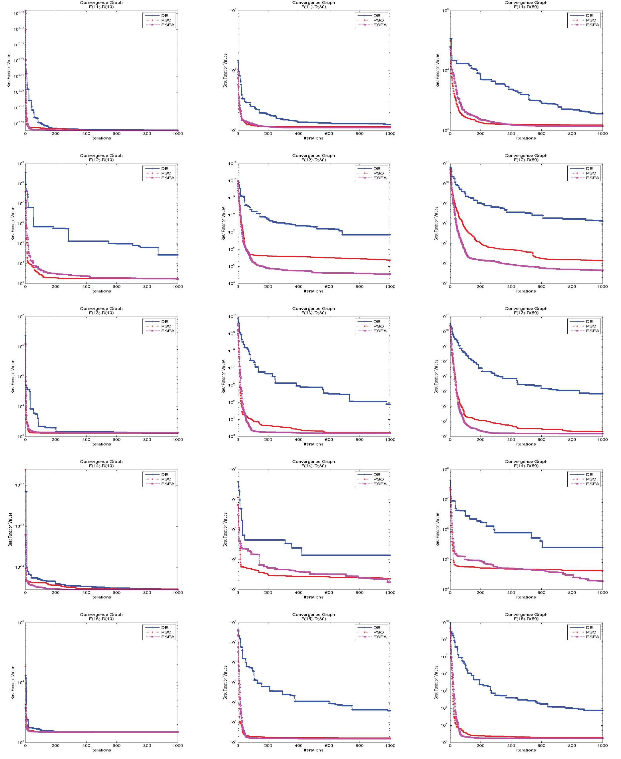
Figure 7 presents the visual convergence graph of the ESEA, PSO, and DE algorithm while solving the benchmark functions from
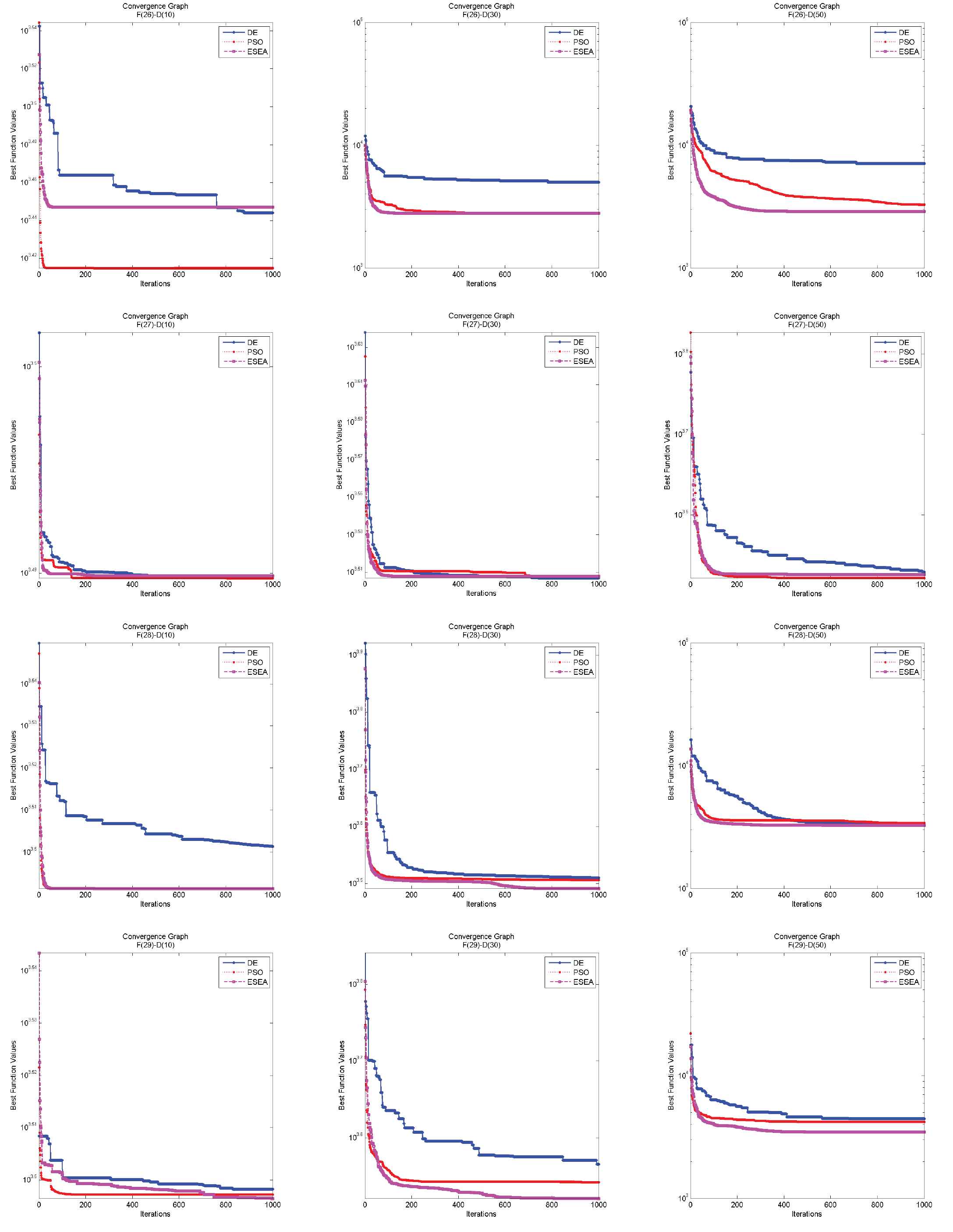
Evolution in the best function values of panel is for problems with fifty dimension.
In Figure 8, the evolution in the average objective function value displayed by ESEA-II versus GA while solving benchmark functions denoted by
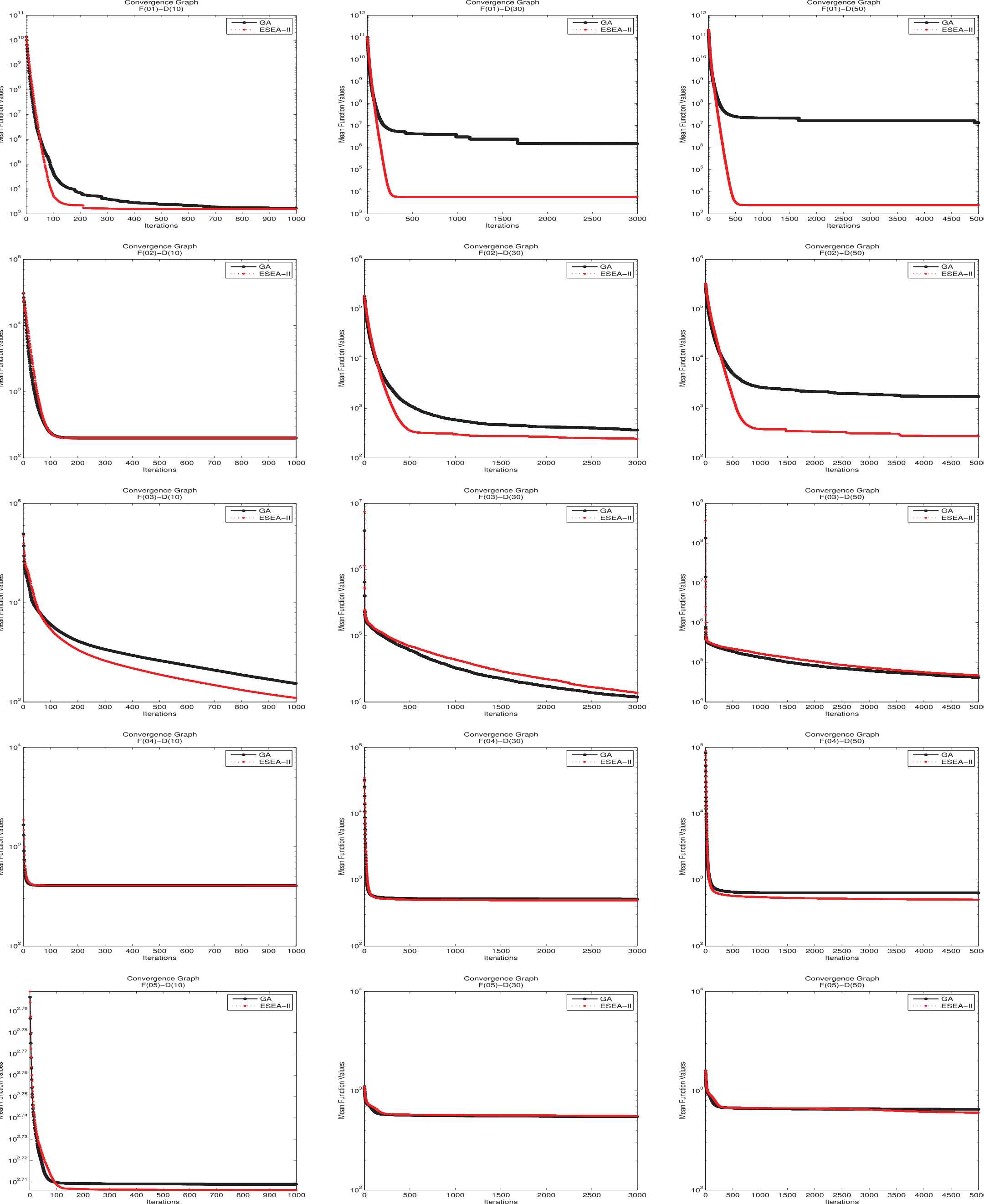
Evolution in the average function values of panel is for problems with fifty dimension.
Figure 9 presents comparison of best function values versus optimal values of benchmark functions
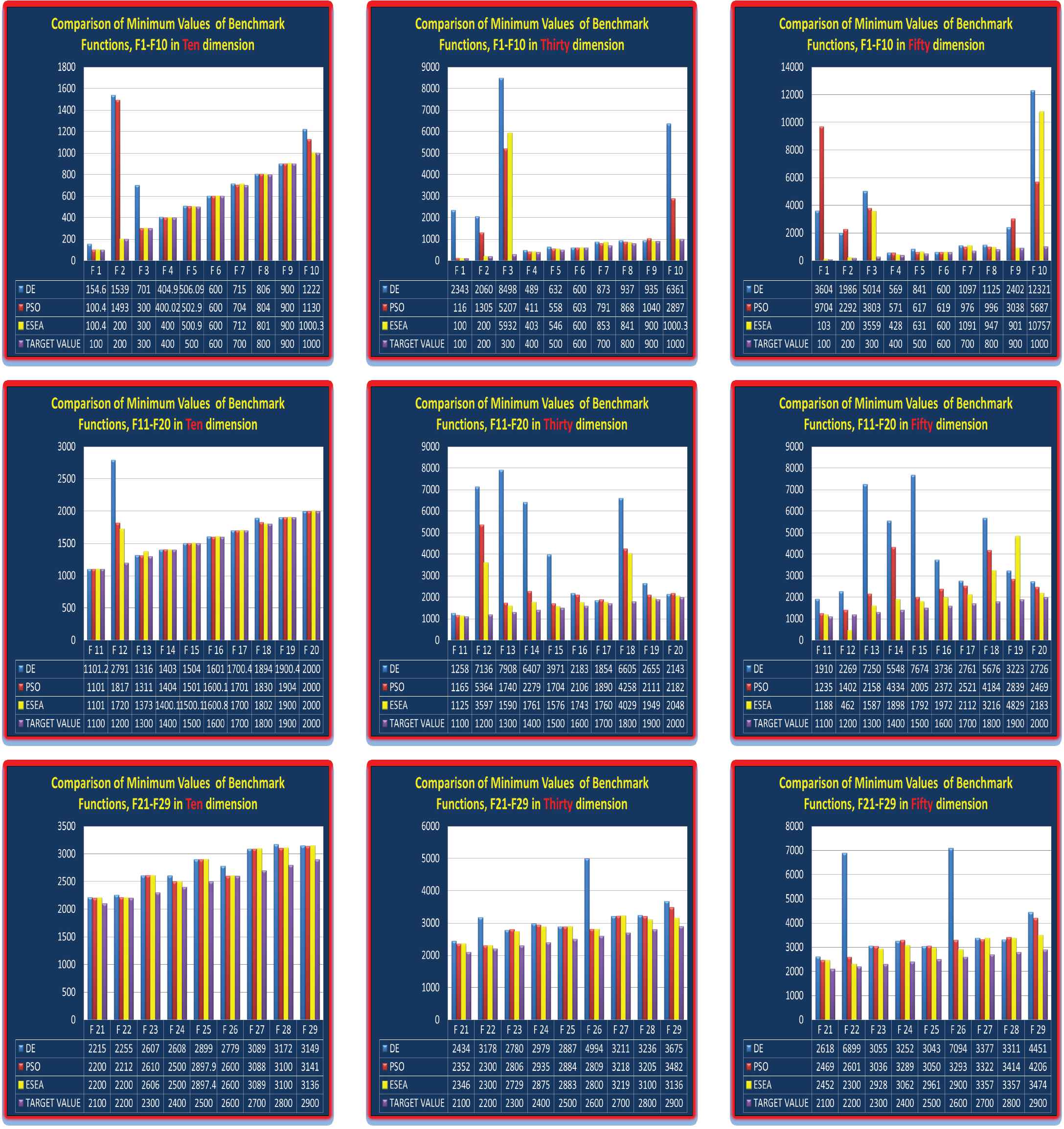
Comparison of best function values versus optimal values of benchmark functions panel is for problems with fifty dimension.
The numerical results as summarized in all tables indicate the consistency of the proposed ESEA algorithm while solving large-scale global optimization problems having had continuous search space. We have also performed the statistical analysis by employing Wilcoxons rank-sum test with
4. CONCLUSION
In the last two decades, EC has played an authoritative role in solving various complex optimization and search problems. A family of EAs under the umbrella of the EC field has many advantages and various distinguishing features as compared to existing traditional mathematical programming techniques while solving complicated optimization problems. EAs have the ability of a collective learning approach, self-adaptation, robustness, and particularly no need for derivative information to conduct their search process. EAs work on a uniformly and randomly generated set of solutions and have been successfully applied to many real-world problems that posed in different disciplines of engineering technologies, business communities, commercial applications. The combined use of different learning techniques might be useful in alleviating the shortcomings of the various baseline EAs in the form of hybridization or fusion of these techniques. Hybrid EAs have a substantial importance in attaining global optimal solutions for the problem at hand as compared to single strategy-based EAs. This paper proposes an ensemble strategy-based EA to solve large-scale global optimization problems with complicated search space. The proposed algorithm so-called ESEA has employed some existing EA as constituent algorithms based on dynamic resources allocation procedure. The constituent algorithms include the PSO, DE algorithm, BA and TLBA, and GA to evolve its population. Promising simulations results have been found by the proposed algorithm over a series of benchmark functions for most of the benchmark functions as compared PSO and DE, and GAs. This good algorithmic behavior of the suggested algorithm is attributed to the intelligent and adaptive strategy of distributed procedure. The proposed algorithm is much flexible and can easily be adapted to a parallel computing network for finding the solution of complicated real-world problems in less computation time. Furthermore, multiple search operators can be assumed in the constituent algorithms in the framework of the proposed algorithm keeping in view the fact that different problems suit different search operators.
In the future, we intend to further investigate the algorithmic behavior of the suggested algorithm upon more complicated benchmark functions and real-world optimization problems.
CONFLICTS OF INTEREST
The authors declare no conflicts of interest.
AUTHORS' CONTRIBUTIONS
The main concept and experimental work were performed by Wali Khan Mashwani and Syed Nouman Ali Shah. The critical revisions and writing, analysis of this manuscript was mainly handled by Wali Khan Mashwani, Syed Nouman Ali Shah along with Abdelouahed Hamdi and Samir Brahim Belhaouari who’s helped us in revising this paper. All authors have reviewed and approved the final manuscript.
Funding Statement
The first two authors are thankful to National Research Programme for Universities (NRPU) Project # 5892 awarded by Higher Education Commission (HEC), Pakistan.
ACKNOWLEDGMENTS
The authors would like to thankful to the referees for their insightful and valuable comments to significantly improve this Manuscript. The authors are highly thankful to Director of Institute of Numerical Sciences, Kohat University of Sciences and Technology for providing all experimental facilities and convenient environment to accomplish this study and successfully completed the NRPU Project 5892.
Footnotes
Ensemble Strategy based Evolutionary Algorithm.
REFERENCES
Cite this article
TY  - JOUR
AU  - Wali Khan Mashwani
AU  - Syed Nouman Ali Shah
AU  - Samir Brahim Belhaouari
AU  - Abdelouahed Hamdi
PY  - 2020
DA  - 2020/12/28
TI  - Ameliorated Ensemble Strategy-Based Evolutionary Algorithm with Dynamic Resources Allocations
JO  - International Journal of Computational Intelligence Systems
SP  - 412
EP  - 437
VL  - 14
IS  - 1
SN  - 1875-6883
UR  - https://doi.org/10.2991/ijcis.d.201215.005
DO  - 10.2991/ijcis.d.201215.005
ID  - Mashwani2020
ER  -