
Emotion Recognition from Speech: An Unsupervised Learning Approach

- DOI
- 10.2991/ijcis.d.201019.002How to use a DOI?
- Keywords
- Emotion recognition; Speech signal; Feature extraction; K-means; Fuzzy clustering; Membership function
- Abstract
Speech processing is quickly shifting toward affective computing, that requires handling emotions and modeling expressive speech synthesis and recognition. The latter task has been so far achieved by supervised classifiers. This implies a prior labeling and data preprocessing, with a cost that increases with the size of the database, in addition to the risk of committing errors. A typical emotion recognition corpus therefore has a relatively limited number of instances. To avoid the cost of labeling, and at the same time to reduce the risk of overfitting due to lack of data, unsupervised learning seems a suitable alternative to recognize emotions from speech. The recent advances in clustering techniques make it possible to reach good performances, comparable to that obtained by classifiers, with much less preprocessing load and even with generalization guarantees. This paper presents a novel approach for emotion recognition from speech signal, based on some variants of fuzzy clustering, such as probabilistic, possibilistic and graded-possibilistic fuzzy c-means. Experiments indicate that this approach (a) is effective in recognition, with in-corpus performances comparable to other proposals in the literature but with the added value of complexity control and (b) allows an innovative way to analyze emotions conveyed by speech using possibilistic membership degrees.
- Copyright
- © 2021 The Authors. Published by Atlantis Press B.V.
- Open Access
- This is an open access article distributed under the CC BY-NC 4.0 license (http://creativecommons.org/licenses/by-nc/4.0/).
1. INTRODUCTION
Nowadays applications are more and more interactive, which requires an optimal human–machine interaction. One of the most obvious ways to achieve this goal is spoken communication. Since a few decades, speech processing has registered considerable progress in different applications, such as speech recognition, synthesis and enhancement, source separation, etc.
Speech is a complex communication form that conveys information at several levels in addition to verbal content. One of these is emotion, a key component that may enable a much more effective interaction. Unfortunately, speech processing applications perform much better for acquiring the verbal content than for the recognition of expressive components. For instance, a benchmark comparison of emotion recognition based on deep learning architectures has shown that emotion recognition is providing accuracy rates under 80% for most expressive speech databases [1]. Furthermore, a recent evaluation of deep learning architectures for emotion recognition on a state-of-the-art expressive speech database, i.e., IEMOCAP [2], has not shown better results [3].
The literature offers approaches that can showcase a very high recognition performance. However, they are usually tested via cross-validation on the same limited-size corpora that are used for their training. It turns out [4] that cross-corpus evaluation is a much more difficult task, with some experimental results bordering random guessing. Due to the high number of parameters characterizing current deep learning models, this appears to be a clear indication that these methods are overfitting, i.e., learning the database rather than its information content. In other words, the good results reported by recent supervised methods on limited-size corpora are not reproducible in different contexts. While the ability of large machine learning models to work well in a regime of overfitting is the subject of current studies [5], this phenomenon cannot be relied upon in the absence of very extensive training sets.
Given the typical size of available corpora, the only alternative approach to avoid overfitting is capacity control, which consists in using machine learning methods whose ability to learn (and thus also overfit) depends on a controllable number of effective parameters. Classic theories developing this approach include Vapnik and Chervonenkis' statistical learning theory, the fat-shattering dimension and Rademacher complexity [6]. However, many methods that do not explicitly refer to these approaches can nevertheless be studied under the framework of complexity control, for instance those based on regularization or stochastic regularization (stochastic gradient descent, early stopping, dropout).
The work described in this paper has the goal to explore the task of emotion recognition from speech signal using a mainly unsupervised workflow. The use of this class of techniques can be justified in the light of capacity control theories, as will be briefly exposed in the following. This gives it an advantage in the reliability of the attained experimental results with limited data.
The methodologies adopted include (a) combined techniques of features analysis, i.e., feature embedding by autoencoders and feature selection by analysis of variance (ANOVA) or mutual information (MI); (b) different clustering methods, such as crisp clustering using K-means, and fuzzy clustering using probabilistic, possibilistic and graded-possibilistic c-means; (c) a novel way to analyze emotion recognition using the sum-of-membership matrix, which is made possible thanks to the use of a possibilistic-type fuzzy clustering, as will be detailed hereafter.
The main contribution of this work consists in proposing a novel methodology for speech emotional content analysis based on clustering, using either crisp or fuzzy methods. The methodology uses unsupervised learning methods, such as autoencoders, to extract features. Up to our knowledge, this is the first work totally relying on unsupervised learning, both for feature extraction and speech clustering. This work is an extension of results presented at the 11th Conference of the European Society for Fuzzy Logic and Technology [7].
The rest of the paper is organized as follows: Section 2 presents the state-of-the-art of emotion recognition from speech, including databases, feature sets, emotion representation models, and the use of unsupervised learning. Section 3 describes the speech materials used in this work, including the expressive speech database chosen, the standard feature set employed and the psychological emotion model adopted. Section 4 details the methods employed for this study. Section 5 reports on the results and the interpretation of the experimental work; finally the conclusion (Section 6) presents some comments and perspectives.
2. RELATED WORK
2.1. Emotion Models
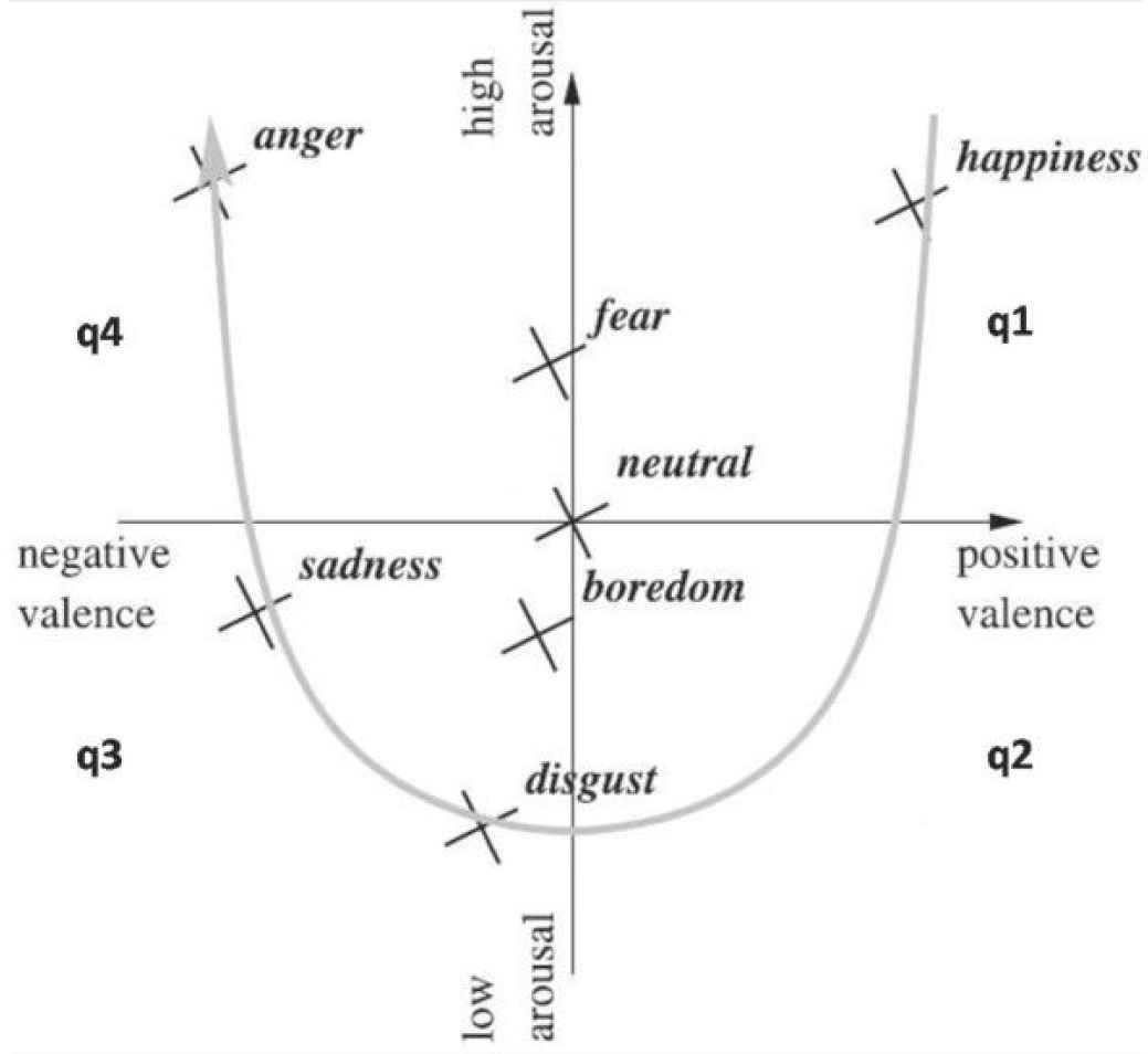
Emotion recognition from speech relies upon established psychological models. For instance, the Ekman model [9] states that there are six basic emotions, i.e., neutral, anger, fear, surprise, joy and sadness, that are recognized whatever the language, the culture or the means (speech, facial expressions, etc.). More detailed models of emotions rely on continuous dimensions rather than atomic “basic” emotions. Russel's circumplex model [10] suggests that emotions can be represented in a bi-dimensional space, where the x-axis represents valence and y-axis represents arousal (cf. Figure 1). Furthermore, Plutchik proposes a tri-dimensional model [11] which combines the basic and the bi-dimensional models. Thus, the outer emotions are a combination of the inner ones.
Classically, and like in speech recognition, emotion recognition was achieved using different methods, namely generative models such as hidden Markov models with Gaussian mixture models (HMM-GMM) [12], artificial neural networks (ANNs) [13,14], and support vector machines (SVMs) [15], yielding nearly the same accuracy [16]. Also, the combination of such models, either in series, in parallel or in a hierarchical way, has given better results than those obtained by single models [16]. Recently, deep learning tools like deep feedforward, recurrent or convolutional neural networks, have outperformed all the aforementioned models for emotion recognition [3,17].
2.2. Emotional Speech Databases
A variety of emotional speech databases were designed or recorded, covering more or less the emotion models described above, i.e., the Eckman [9], Russel [10] and Plutchik [11] models. An inventory of emotional speech databases [16] shows that the main differences between them lie in (a) the size, varying from a few tens of sentences to a few thousands [18]; (b) the number of speakers; (c) the type of speech, whether uttered by professional actors, or recorded from spontaneous conversation like telephone recordings; and (d) the number of emotions, which depends on the emotion model. A recent and updated comprehensive inventory [19] lists the main emotional speech databases. In particular, the EMO-DB database [20] has been widely used, since it covers all basic emotions in equal and sufficient proportions.
2.3. Standard Emotion-Recognition Features
Whatever the chosen model of emotions, a speech signal provides a representation of it that lies at a much lower level, i.e., a train of audio samples (see Figure 2). Therefore, special importance should be given to intermediate representations that make it possible to discriminate the types of emotional content; in other words, features have a crucial importance.
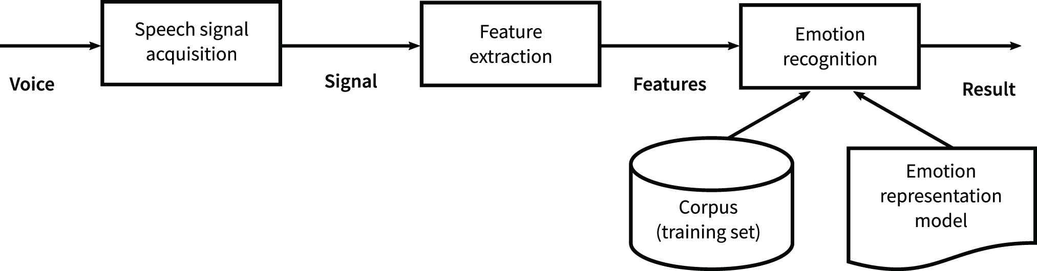
General scheme of an emotion recognition system.
In machine learning there are two main approaches to obtaining good features: Using standard, expert-engineered feature sets that are known to be well correlated with the desired recognition task; or using optimization to learn features that will provide the best performance. In this work we will adopt both approaches, by encoding speech signals using standard feature sets at the lower level, but subsequently extracting higher-level features by means of unsupervised learning.
Generally in speech recognition the commonly used features can be divided into prosodic vs. acoustic (or spectral) ones. Prosodic features include
Another classification of features relies on the level of extraction, i.e., local vs. global features. Local features are extracted at each frame, like
2.4. Feature Learning Methods: Extraction and Selection
The ultimate goal of feature analysis is to optimize the input space, either by discarding the irrelevant (or redundant) features, i.e., feature selection, or by a nonlinear combination of features in order to obtain more discriminant ones, i.e., feature extraction. In particular, one interesting technique for feature extraction is feature embedding.
In the particular case of emotion recognition, feature analysis, either by extraction or by selection, has been widely used. For instance, feature extraction by sequential format floating search (SFFS) was used to choose the most relevant features for emotion recognition based on Bayesian classification [24]. The SFFS criterion was applied with the assumption that the features follow a multivariate Gaussian distribution. Then the variance of the correct classification rate of the Bayesian classifier during cross-validation is estimated.
Also, principal component analysis (PCA) was used in several emotion recognition-related works [25–28]. For emotion recognition, it has been noticed that the classification accuracy increases when the number of principal components is increased up to a certain order, after which the accuracy starts to decrease [16].
Albeit to a lesser degree, linear discriminant analysis (LDA) was also used in some works about emotion recognition. However, the results about the relevance of each group of features, i.e., pitch-related, energy-related and spectral features are not coherent enough [16]. This may be due to the difference of databases and feature sets used in each work.
To compare PCA and LDA for emotion recognition, both techniques were applied on BHUDES, a Chinese emotional speech corpus [29], before undertaking classification with ANN and SVM [30]. For both classifiers, the results have shown that using LDA for feature selection gives better recognition rates than using PCA, either for all classes or for every single emotion.
Furthermore, Eyben et al. evaluated the feature relevance in real-life conditions [31]. To fulfill that, an experience was set up by corrupting clean speech by different noise level, before extracting the standard ComParE feature set [32]. Then the Pearson correlation coefficients (CCs) of each feature with continuous target label was computed. The selected features were the subset of 400 features (among 6353 ones) having the best CC coefficients for arousal, valence and level of interest (LOI) tests. However, it has been shown in the tests that change in feature group relevance depends more on the individual tests than on the level of noise.
The feature extraction methods described so far, PCA and LDA, are linear mappings which make strong assumptions about the structure underlying the data. An alternative approach is nonlinear feature embedding.
The autoencoder is a neural network whose objective approximates the identity function. It is commonly used as an unsupervised learning technique, that aims to extract features from unlabeled data. To achieve this goal, the autoencoder optimizes the weights to minimize the mean square difference between the given input and the obtained output; then, the value of a hidden layer is used as an encoded representation of the input.
As shown in Figure 3, a simple autoencoder has only one hidden layer. It is therefore parameterized by weights (
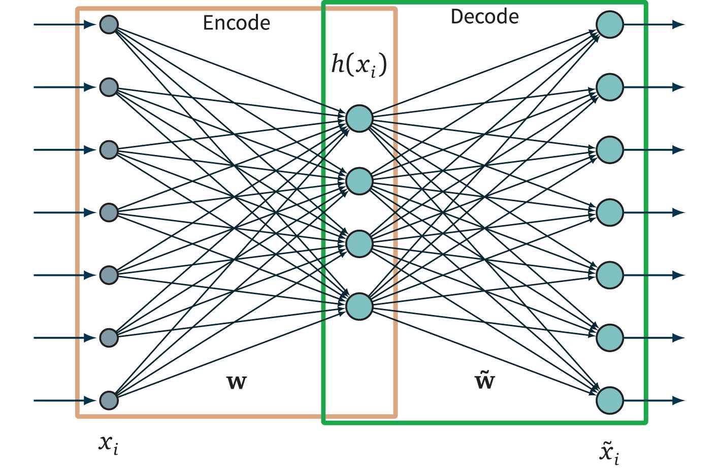
Autoencoder architecture.
It can be shown that the encoding obtained from a simple linear autoencoder, i.e., with
Deep autoencoders with several hidden layers are also possible, although this may imply an excessive overparameterization with increased risk of overfitting, or, correspondingly, the need for exponentially more data.
A simple autoencoder can be split into two parts: (a) the encoder, from the input layer to the middle layer and (b) the decoder, from the middle layer to the output layer. The encoded features are obtained at the output of the encoder layer. Hence, to reduce the dimension of the input space, the encoder layer should have a lower dimension than the input layer (cf. Figure 3). The encoder layer provides a useful transformation of input features, that allows, first discovering hidden structure in the input features, and second generating new features through the nonlinear transformation of the input features by the activation functions of the hidden layers.
The autoencoder has been used as a feature extraction method in several clustering-based works. For instance, Song et al. [34] trained an autoencoder with a new objective function, where the centroids are updated at the same time as the weights and biases of the neural networks. In the work of Xie et al. [35], clustering was based on deep autoencoders. This process starts by initializing the parameters of the clustering model with an autoencoder, and then the centroids and the autoencoder's parameters are optimized using Kullback–Leibler (KL) divergence to maximize the similarity between the distribution of the embedded features and the centroids. A comparison between using or not autoencoded features for spectral clustering was conducted on different data sets [36], such as documents (20-Newsgroup), biological data (DIP [37] and BioGrid [38]) and chemical data (WINE [39]), to reveal that the autoencoded features yield better results.
2.5. Clustering
Clustering techniques can be inventoried following several criteria, whether they are hierarchical, partition-based, density/neighborhood-based or model-based [8]. Obviously clustering was less used than classification for emotion recognition, since most works deal with labeled databases. However, in a big data context, unsupervised recognition methods can prove more useful, since labeling a huge quantity of expressive speech data would be a tedious and expensive task.
For instance, self-organizing maps (SOMs) were used by Szekely et al. to detect emotions in audiobooks [40], based on articulatory features. Also, hierarchical K-means were used by Eyben et al. to detect emotions in a corpus dedicated for expressive speech synthesis, using prosodic and acoustic features [31]. It should be noted that, since clusters do not necessarily correspond to classes, a “vector quantization” approach is usually used, whereby the number of clusters is overestimated, and subsequently the detected clusters are grouped into classes; methods based on this type of approach can even be competitive with entirely supervised approaches, with theoretical guarantees [41], and can be easily used in a semi-supervised context (partially labeled data).
Experiments have shown that in clustering the choice of features is more important for the final accuracy than in classification, where the generalization power of the classifier and the direct minimization of a loss function could mask the irrelevance or the aberrance of some features.
In this work, we are particularly interested in applying some of our recent results in fuzzy clustering [42] for emotion recognition. The soft/fuzzy clustering approach consists in using a real-valued membership function instead of a categorical or binary membership decision. Then an object belongs to all clusters, but with different membership degrees, having values between 0 and 1 [43].
The fuzzy clustering problem can be stated as follows: Given a set
Considering the membership function, fuzzy clustering methods can be categorized as either probabilistic or possibilistic. Then the pair
A possibilistic partition if
A probabilistic partition if it is a possibilistic partition such that
The extremely popular central clustering approach consists in defining clusters
All fuzzy versions of K-means are in principle based on minimizing the following objective function:
However, directly minimizing this objective yields a degenerate problem, whose solution is given by the (crisp) K-means method. For a real-valued (i.e., fuzzy) solution, the distortion objective is regularized in either of two ways, which were proved to be related by a common framework [44]: Either by introducing an exponent
Optimization of the objective is customarily done via alternate minimization, which iteratively solves two problems assumed as independent: minimization with respect to centroid positions and minimization with respect to memberships.
In all cases, the cluster centroids
Regarding the membership function, in the cases of our interest it can be expressed as
Regarding the generalized partition function
The fuzziness parameter
3. SPEECH MATERIAL
To perform this work, an emotional speech database was selected from the available speech corpora. We chose EMO-DB [20] since it has been widely used and cited as a reference. Besides, a special attention was addressed to choosing the feature set, since several ones have been proposed in the literature.
3.1. Speech Database
EMO-DB [20] is a publicly available database of prepared emotional speech. Prepared speech corpora differ from spontaneous speech corpora, since they are elaborated by linguists to represent all the language phenomena in a balanced and normalized way. EMO-DB contains 10 German sentences (5 short and 5 long) uttered by 10 native-speaking professional actors (5 male and 5 female). Every sentence was uttered by every actor in 7 emotions (neutral, anger, boredom, fear, disgust, joy and sadness) once (or twice in a few cases). The sentences were recorded in an anechoic chamber, at 16 KHz sampling rate. The database was labeled including the emotion of each sentence, the syllabic segmentation and the stress level of each syllable. It is worth noting that EMO-DB has provided the highest emotion recognition rates using state-of-the-art classifiers, such as HMM-GMM and SVM [21].
3.2. Feature Set
Emotion recognition feature sets have been addressed extensive research, yielding a variety of proposed sets [19]. However most feature sets used a limited number of feature types, i.e., prosodic, spectral, voice-quality-related [19] and in a lesser proportion articulatory features [40]. Furthermore, the global features, i.e., statistics calculated all over the speech signal, were generally preferred to local features that are measured at each frame [50]. In particular, The Interspeech'09 emotion recognition challenge feature set was preferred to conduct this work, for two main reasons: (i) its preliminary results [21] and (ii) its compactness. Then features were extracted using the Opensmile toolkit [51]. Tables 1 and 2 show the complete set of features and the calculated statistics extracted for each, respectively, so that 384 features (16 descriptors + their 16
| Speech Parameter | Descriptors |
|---|---|
| Zero-crossing rate | ZCR, |
| Root mean square energy | RMS energy, |
| fundamental frequency | |
| Harmonic-to-noise ratio | HNR, |
| 12 Mel-Frequency cepstral coefficients | (MFCC (1–12)), |
Interspeech'09 emotion recognition challenge feature set.
| Features for Each Descriptor | Parameters |
|---|---|
| Global statistics | Mean, standard deviation, skewness, kurtosis |
| Minimum | Value, relative position, range, |
| Maximum | Value, relative position, range, |
| Linear regression coefficients | Offest, slope, Mean square error (MSE) |
Statistical parameters used for Interspeech'09 emotion recognition challenge feature set.
3.3. Emotion Classes
Initially, classes consisted in single emotions, namely neutral, anger, boredom, disgust, fear, joy and sadness. However, we also employed a second way to label speech signals by using groups of emotions as classes instead of individual emotions. In fact, grouping emotions using the valence/arousal mapping was thought to increase clustering performance (cf. Table 3). Both sets of labels were evaluated during experiments.
| New Label | Grouped Labels | Common Characteristics |
|---|---|---|
| AJ | Anger and Joy | High absolute valence and arousal |
| NB | Neutral and Boredom | Low absolute valence and arousal |
| FD | Fear and Disgust | Low absolute valence and medium absolute arousal |
| S | Sadness | High absolute valence and medium absolute arousal |
Groups of emotions.
4. METHODS
To conduct the experimental process, different steps were followed. First, the speech corpus was preprocessed to extract and select the most relevant features, second crisp and fuzzy clustering were performed following different strategies, third clusters were majority-labeled with class labels and finally the clustering and classification results were analyzed (cf. Figure 5).
4.1. Preprocessing
The experimental process starts with a preprocessing phase, in which the following steps are performed: (a) feature embedding, where the original descriptors (cf. Tables 1 and 2) were transformed by embedding with the autoencoder, so that a new set of features was extracted; (b) feature selection, where the final features were selected amongst the extracted ones, using either ANOVA or MI test.
4.1.1. Feature extraction
The first step in feature analysis consists in feature extraction. In this work, it was performed through feature embedding using a 3-hidden-layer deep autoencoder. The set of 384 features for each signal (cf. Table 1) is trained by the autoencoder to extract a smaller number of features at the encoder layer. Therefore, two schemes of preprocessing were tried out: (i) application of the autoencoder to the whole set of features and (ii) application of the autoencoder to each low-level descriptors (LLD) group, so that only one feature is extracted out of each 12-feature LLD. The autoencoder architectures used in (i) and (ii) are described in Table 4.
| Input Ffeatures | Input Layer | Hidden Layer 1 | Code Layer | Hidden Layer 3 | Output Layer |
|---|---|---|---|---|---|
| All features | 384 | 500 | 32 | 500 | 384 |
| LLD features | 12 | 100 | 1 | 100 | 12 |
Autoencoder architectures (layers and number of nodes).
4.1.2. Feature selection
Once the features were extracted, through embedding, feature selection was set up. Although features seem to be mostly uncorrelated, a finer analysis was performed using ANOVA and MI to further reduce the cardinality of the set of extracted features. Furthermore, to keep a certain coherence between the selected features, two ANOVA strategies were adopted, the first evaluating individual features, and the second, denoted ANOVA group, evaluating groups of features, where each group contains the 12 statistics of each descriptor (cf. Tables 1 and 2).
4.2. Clustering
4.2.1. The graded possibilistic C means algorithm
As well as using the “crisp” K-means clustering method, we will follow a fuzzy approach by employing the graded-possibilistic c-means (GPCM) algorithm for unsupervised learning.
The graded-possibilistic paradigm [48] allows to switch continuously between the probabilistic and possibilistic paradigms by modulating the free parameter
Also, it is worth noting that in case of probabilistic central clustering,
To calculate the values for the cluster width parameters
4.2.2. Use of possibilistic membership for classification analysis
A distinctive advantage of the possibilistic paradigm, as compared to “probabilistic” fuzzy clustering, is represented by the ability to evaluate the typicality of patterns with respect to the learned clusters. Since memberships are not constrained to have a constant sum, for a given data instance it is possible to analyze the sum-of-memberships to each cluster and evaluate how well it fits the clusters distribution.
It is also possible to analyze the cumulative sum-of-memberships by classes, to gain insight on the “perceived” internal structure of emotions, to check for instance if two emotions are consistently considered similar. This particular analysis will be presented for the experimental results in Section 5.
From the technical standpoint, the graded approach used in this work partially constrains the sum-of-membership; one advantage of this is ruling out degenerate solutions, and another one is allowing for an easier convergence of the optimization. However, the cumulative sum-of-membership matrix will have entries that depend on the degree of probabilistic tendency
4.2.3. Parameter setting
In Rovetta et al. [42] it was observed that
4.3. Capacity Control in Unsupervised Learning
Now we provide a brief justification of the choice of supervised learning for limited-size data sets. The learning capacity of a central clustering model followed by supervised labeling was studied in a previous work [41]. In particular, the Vapnik–Chervonenkis dimension of this class of learning methods was established by Theorem 1 from the reference.
Theorem 1.
[41] The Vapnik–Chervonenkis dimension of a central clustering model with
The significance of this theorem, whose proof can be found in the referenced paper, lies in the fact that the only free parameter that influences the learning capacity is the number of centroids, so neither the dimensionality (number of features) nor the size (number of observations) of the data influence the Vapnik–Chervonenikis dimension. This capacity measure is computed in a worst-case scenario, so it is an overestimation of the actual learning capacity that can be expected in real cases. If we can upper-bound the Vapnik–Chervonenkis dimension, we can be confident that other, more realistic indexes like the fat-shattering dimension will not exceed it.
5. EXPERIMENTAL WORK
5.1. Experimental Protocol
Experiments were carried out following a protocol where the model parameters were varied, one at a time:
The labels set, i.e., single emotions or groups of emotions (cf. Table 3).
The number of clusters, increasing from the number of classes, to 3 times.
The feature selection method, i.e., ANOVA or MI.
The number of selected features, decreasing from all features, i.e., no feature selection, to
These combinations yielded a high number of experiments, therefore only those providing the most relevant results are presented (cf. Table 5). In addition, at every execution of the fuzzy clustering algorithms, K-means was performed under the same conditions, i.e., number of classes, number of clusters, feature selection method and the number of selected features, and using a fixed number of replicates, equal to 10.
| Number of Classes | Number of Clusters | Feature Selection Method | Proportion of Selected Features (%) | K-means Rate (%) | GPCM Rate (%) | ||
|---|---|---|---|---|---|---|---|
| 7 | 7 | ANOVA group | 50 | 0.1 | 0.9 | 51.9 | 69.6 |
| 7 | 14 | ANOVA | 25 | 0.1 | 0.9 | 56.6 | 55.9 |
| 7 | 21 | ANOVA | 25 | 0.1 | 0.9 | 60.9 | 63.0 |
| 4 | 4 | ANOVA | 75 | 0.1 | 0.9 | 62.4 | 61.3 |
| 4 | 8 | ANOVA | 50 | 0.1 | 0.9 | 69.9 | 77.4 |
| 4 | 12 | ANOVA | 50 | 0.1 | 0.9 | 73.9 | 75.1 |
Best recognition rates (in bold character) for different parameters combinations.
5.2. Results
Figure 4 shows a representation of clusters, projected in 3D using PCA as a visualization tool, for the original clusters, whereas Figure 6 shows the 2D distribution for predicted clusters using different methods, i.e., K-means, probabilistic, possibilistic and graded-possibilistic c-means.
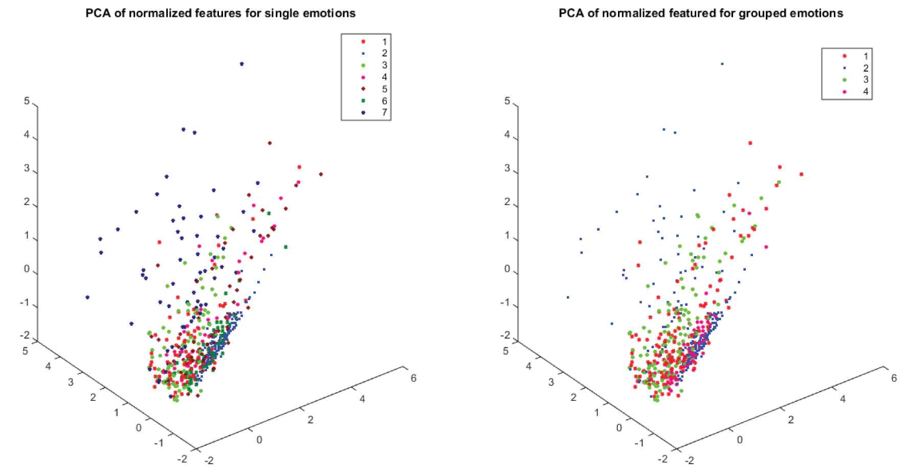
Distribution of single and grouped emotion classes, visualized using principal component analysis (PCA) to project features in three dimensions: (a) for single emotions, three-dimensional projection suggests that the Interspeech'09 standard features are not discriminatory enough and (b) emotions were grouped the reduce feature scattering.
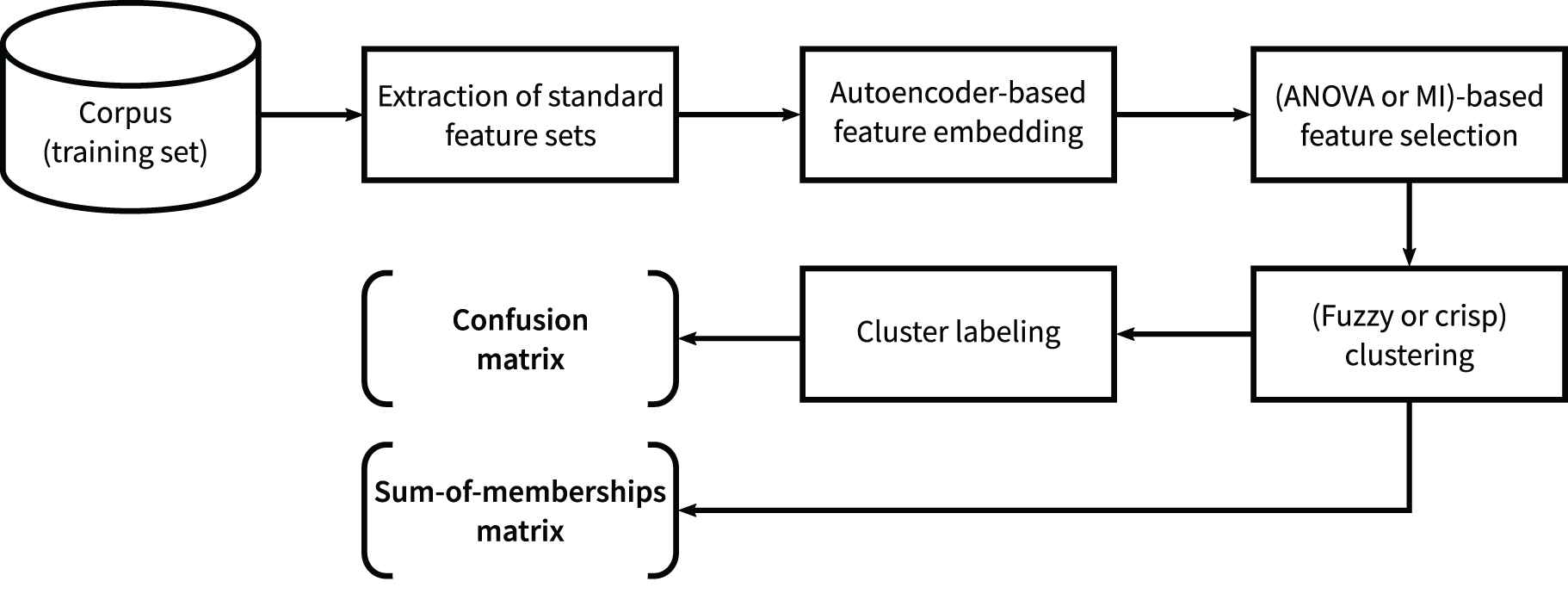
Experimental process as applied in this work: Preprocessing includes hand-crafted feature computation, feature embedding and selection; clustering is achieved using crisp (K-means) and/or fuzzy methods, cluster labeling is applied to recuperate emotion classes from clusters. The evaluation outputs are the confusion and the sum-of-membership matrices.
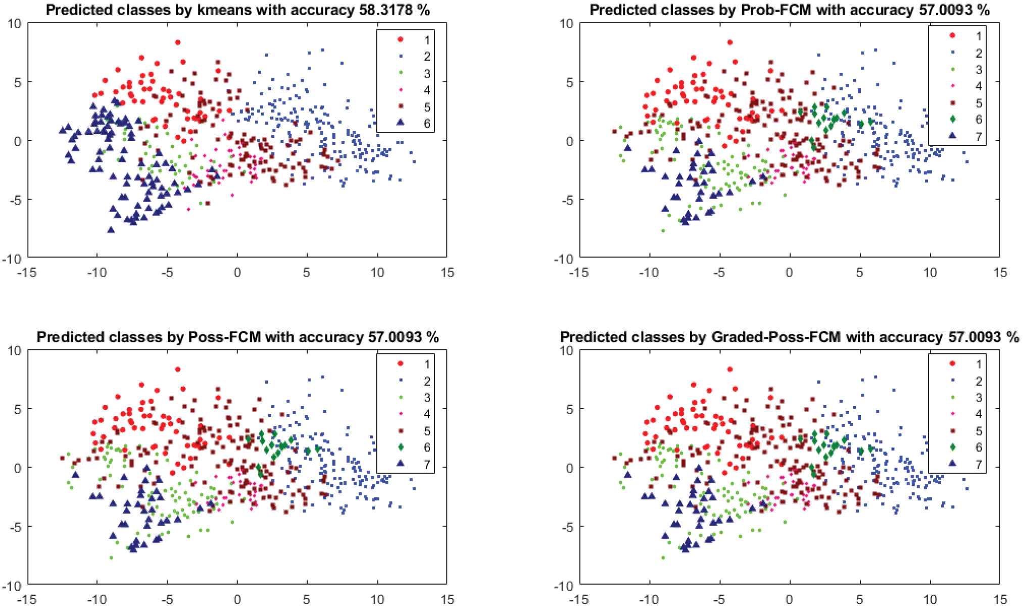
Clustering results for 7 classes using 21 clusters and 96 features selected by analysis of variance (ANOVA) method for K-means and different graded-possibilistic c-means (GPCM) methods (two-dimensional principal component analysis (PCA) projection): Though the two-dimensional projection does not show clearly disjoint clusters, K-means and GPCM methods seem able to separate some classes, e.g., Class 1 and Class 2.
5.2.1. Confusion matrix
The performances of both crisp and fuzzy clustering, followed by supervised labeling, were analyzed through the scores calculated from the confusion matrix, i.e., overall accuracy, precision, recall and F1-score (cf. (6a) to (6d)).
5.2.2. Sum-of-membership matrix
This proposed matrix (cf. Table 6) shows, for every recognized emotion class, the sum of the memberships to original classes. The coefficients of this matrix correspond to the sum-of-membership to an original class, calculated for all samples. This method is proposed in order to measure how many emotion classes were correctly recognized, or in other terms how much the features of every single emotion are shared by the other ones. The matrix can be analyzed like a confusion matrix, where the lines correspond to the recognized emotions and the columns to the original ones.
| Classes | Neutral | Anger | Boredom | Disgust | Fear | Joy | Sadness |
|---|---|---|---|---|---|---|---|
| Neutral | 35.1571 | 5.0713 | 23.3220 | 5.1520 | 6.3261 | 2.7159 | 6.9717 |
| Anger | 5.2943 | 60.7539 | 3.9122 | 3.8892 | 9.9439 | 27.4724 | 0.1005 |
| Boredom | 6.0872 | 2.7400 | 17.6296 | 6.7532 | 4.8307 | 1.9224 | 17.0275 |
| Disgust | 9.3078 | 6.3142 | 10.6536 | 12.7571 | 5.9771 | 4.7399 | 0.5343 |
| Fear | 16.0078 | 28.1121 | 15.1840 | 11.4498 | 35.0615 | 12.5662 | 11.8798 |
| Joy | 0.5790 | 18.8198 | 0.1959 | 0.7331 | 2.8752 | 18.7432 | 0.0006 |
| Sadness | 6.5668 | 5.1887 | 10.1028 | 5.2657 | 3.9855 | 2.8400 | 25.4855 |
Sum-of-membership matrix calculated using 192 features selected by MI, GPCM with
5.2.3. Initial distribution of classes
It looks since the beginning that in spite of using a standard feature set [21], the distribution of classes looks too dispersed (cf. Figure 4).
5.2.4. Fuzzy clustering performance
However, thanks to feature embedding and then feature selection, and to a good choice of the possibilistic and graded-possibilistic models parameters, i.e.,
5.2.5. Single emotions vs. groups of emotions
Another result consists in increasing the clustering rate when emotions were grouped using the valence/arousal model. This could be explained by the fact that using more samples and less classes may increase the clustering rate, but it also tells about the relevance of grouping such emotions, despite some pairs contain opposite emotions (e.g., anger and joy). This last point may be useful in emotion analysis, using objective measures, such as the statistics used in the feature set.
5.3. Benchmarking
In order to compare the performance of the proposed approach, the results of other methods applied on the same expressive speech database, i.e., EMO-DB [20], have been investigated. Table 8 shows the highest overall accuracy measured for such methods, combining supervised and unsupervised techniques for feature extraction and classification. It looks that the proposed approach, entirely based on unsupervised learning, both for feature extraction and classification, is not far away from the other methods that use supervised learning, either partly (for classification only) or entirely (in the whole process).
| Learning | Input Features | Feature Extraction | Classification | Accuracy (%) |
|---|---|---|---|---|
| All supervised | Spectrogram images | CNN | BLSTM [52] | 91.3 |
| Raw audio | CNN | LSTM [17] | 88.9 | |
| Unsupervised feature | Spectrogram images | K-means | SVM [53] | 71.5 |
| extraction and | Spectrogram images | Autoencoder | SVM [53] | 67.4 |
| supervised classification | ||||
| All unsupervised | Interspeech'09 [21] | Autoencoder | K-means-VQ (Prop) [7] | 60.9 |
| Interspeech'09 [21] | Autoencoder | GPCM-VQ (Prop) [7] | 69.6 |
Benchmark results of different methods combining supervised and unsupervised feature extraction and classification on EMO-DB expressive speech database (n.b. CNN: Convolutional neural networks, LSTM: Long short-term memory, BLSTM: Bidirectional long short-term memory, SVM: Support vector machines).
5.4. Interpretation and Discussion
In addition to emotion recognition, further results could be obtained from analyzing the results obtained by fuzzy clustering under the possibilistic framework. In the following we the confusion and the sum-of-membership matrices could provide as novelty regarding emotion analysis.
5.4.1. Analysis of the classification results
Though the obtained classification results may be lower than those that should have been provided by supervised learning, the obtained rates can be considered as satisfactory in the framework of unsupervised learning. In fact, cluster labeling has been utilized in this work only to check the performance. However, in real-world application of the proposed method, the data need not be entirely labeled, hence obtaining an overall accuracy of about 60% might be encouraging. A deeper analysis of the classification scores (cf. Table 7 and Figure 7) shows that: (a) crisp and fuzzy clustering do nearly the same for each class of emotions, e.g., anger and sadness are both well recognized, whereas joy is much less predicted by both techniques, though all classes have the same number of samples; (b) F1-score is higher than 50% for most emotion classes and for both methods, i.e., crisp and fuzzy clustering, which means that precision and recall are rather balanced (though it is less obvious for some emotions like disgust and joy). In fact the F1-score is a measure that reveals whether a high accuracy could hide unbalanced precision and recall.
| K-means |
GPCM |
||||||||||||||
|---|---|---|---|---|---|---|---|---|---|---|---|---|---|---|---|
| Original Classes |
|||||||||||||||
| Neutral | Anger | Boredom | Disgust | Fear | Joy | Sadness | Neutral | Anger | Boredom | Disgust | Fear | Joy | Sadness | ||
| Pred. Classes | Neutral | 50 | 0 | 18 | 5 | 14 | 6 | 1 | 36 | 0 | 5 | 3 | 10 | 6 | 2 |
| Anger | 5 | 115 | 2 | 3 | 12 | 46 | 0 | 5 | 112 | 1 | 3 | 11 | 47 | 0 | |
| Boredom | 12 | 0 | 42 | 11 | 1 | 2 | 8 | 25 | 0 | 48 | 11 | 3 | 2 | 6 | |
| Disgust | 2 | 0 | 1 | 21 | 6 | 2 | 1 | 0 | 0 | 1 | 17 | 3 | 2 | 0 | |
| Fear | 7 | 5 | 4 | 6 | 32 | 7 | 0 | 9 | 8 | 8 | 12 | 40 | 6 | 4 | |
| Joy | 0 | 7 | 0 | 0 | 1 | 8 | 0 | 0 | 7 | 0 | 0 | 1 | 8 | 0 | |
| Sadness | 3 | 0 | 14 | 0 | 3 | 0 | 52 | 4 | 0 | 18 | 0 | 1 | 0 | 50 | |
Confusion matrices calculated by K-means and GPCM, both with subsequent cluster labeling, using 192 features selected by ANOVA and with GPCM parameters
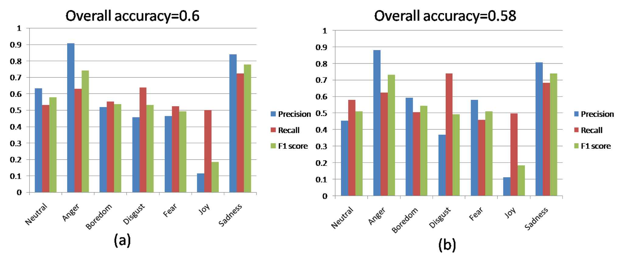
Scores of the confusion matrix for (a) K-means, (b) graded-possibilistic c-means (GPCM), for clustering followed by labeling, using 192 features selected by analysis of variance (ANOVA).
Finally, though emotion classes are balanced in the EMO-DB database [20], the differences between classification results may be due to the choice of features. Though we opted for a standard feature set, that has been successfully used for Interspeech'09 emotion recognition challenge [21], it looks less efficient to detect all emotions equally. Another interpretation could be that some intense emotions, such as joy, may share a lot of their aspects like valence and arousal, and hence have similar features as other emotions that have similar levels of valence or arousal, such as anger.
As noted in Section 4, the sum-of-membership matrix provides a way to analyze these aspects.
5.4.2. Analysis of the sum-of-membership matrix
By inspecting the sum-of-membership matrix (Table 6), in line 2 the recognized emotion anger has the highest sum-of-membership to the same original emotion, which means that most samples recognized as belonging to the class anger have the highest membership value to the same class. This is also the case for classes neutral and sadness. However, for the other recognized emotions, like boredom, disgust, fear and joy, the sum-of-membership matrix shows that their sum-of-membership to some other classes are as high as for the original classes, e.g., the recognized class boredom shares nearly the same sum-of-membership to the original classes boredom and sadness, and recognized joy shares the same sum-of-membership with original joy and anger, etc.
In comparison to the scores calculated from the confusion matrix, cf. Figure 7, it could be easily noticed that highly misclassified emotions are the same which share most of their membership functions with other ones, such as disgust and joy. Hence, the sum-of-membership matrix could show the same tendency of the confusion matrix in case of fuzzy clustering. These findings could be interpreted as a novel way to approach emotion recognition/perception, e.g., when a recognized emotion class has most of its memberships in the same original class, e.g., for anger, this means that the model succeeds to identify most of the angry voices as belonging to the same class; however, when a recognized class has its sum-of-membership shared by more than one original emotion class, this could be interpreted, either as these classes share several features, e.g., for joy and anger, or the emotion itself is a mixture of more basic ones, e.g., disgust is a mixture of anger, boredom and neutral. Still, this interpretation could be deepened by human-listeners through subjective evaluation. At last, such an analysis shows the relevance of fuzzy clustering in (i) enhancing the emotion recognition from single signals, (ii) analyzing emotions, or at least to reveal some of their hidden characteristics thanks to the analysis of the sum-of-membership matrix.
6. CONCLUSION
In this paper, a novel approach for emotion recognition using fuzzy clustering is described. The main idea consists in clustering speech according to basic emotions, using (a) unsupervised learning for feature extraction, and more precisely feature embedding with autoencoders, (b) new advances in fuzzy clustering, such as possibilistic and graded-possibilistic c-means, in addition to probabilistic c-means, to recognize emotion from speech. Besides, the crisp approach was treated using K-means algorithm, for evaluation purposes. Several adjustments were also made to fine-tune the models, including feature embedding using autoencoders, feature selection using ANOVA and MI analysis, and finally varying the possibilistic models parameters. Also, using more clusters than classes helped increasing the recognition rates. In addition, choosing the optimal values of parameters had an impact on increasing the performance of possibilistic and graded-possibilistic c-means models.
The confusion matrix scores, i.e., accuracy, precision, recall and F1, confirm the efficiency of using fuzzy clustering as an alternative tool to supervised learning for emotion recognition. Either for single emotions or for groups of emotions, crisp and fuzzy clustering perform almost equally, yielding an overall accuracy of nearly 60% and a precision higher than 80% for some emotions such as anger and sadness, with equivalent recall. This may be quite useful as an alternative way for emotion recognition in large and especially unlabeled speech data sets.
In addition to the classical confusion matrix, utilized to show the classification performance, a novel representation based on the sum-of-membership matrix is presented. The analysis of such a matrix for fuzzy clustering shows a similar behavior than the confusion matrix, where highly recognized emotions tend to have a high membership to the same original emotion, whereas misclassified emotions tend to share their sum-of-membership with other emotions. This already allows differentiating between “strong” or “basic” emotions, which monopolize their membership values and “weak” or “mixed” emotions that tend to share their sum-of-memberships. This representation allows studying the dependence of each basic emotion to the other ones, and could be a helpful tool for emotion analysis, to understand how speech signal conveys emotions and how they are perceived.
ACKNOWLEDGMENTS
This work was supported by the research grant funded by “Fondi di Ricerca di Ateneo 2016” of the university of Genova. The authors declare that there is no conflict of interest regarding this work. Author 1 and author 2 have contributed equally to this work; author 3 and author 4 have contributed to the revision of the article.
REFERENCES
Cite this article
TY  - JOUR
AU  - Stefano Rovetta
AU  - Zied Mnasri
AU  - Francesco Masulli
AU  - Alberto Cabri
PY  - 2020
DA  - 2020/10/29
TI  - Emotion Recognition from Speech: An Unsupervised Learning Approach
JO  - International Journal of Computational Intelligence Systems
SP  - 23
EP  - 35
VL  - 14
IS  - 1
SN  - 1875-6883
UR  - https://doi.org/10.2991/ijcis.d.201019.002
DO  - 10.2991/ijcis.d.201019.002
ID  - Rovetta2020
ER  -