
An Extended Three-Stage DEA Model with Interval Inputs and Outputs
- DOI
- 10.2991/ijcis.d.201019.001How to use a DOI?
- Keywords
- Three-stage DEA model; Interval DEA; Degree of efficiency change; Improvement benchmark
- Abstract
The traditional three-stage data envelopment analysis (DEA) model only measures exact input–output indicator data, but cannot perform efficiency analysis on uncertain data. The interval DEA method does not exclude the influence of external environmental factors. Therefore, this paper combines the traditional three-stage DEA model with the interval DEA method, and proposes a three-stage interval DEA efficiency model, which eliminates the impact of external environmental factors and realizes the measurement of the efficiency for interval data. From the perspective of the impact of environmental factors, defining the degree of efficiency change vector, a clustering analysis technique based on the efficiency change degree vector is proposed to provide improvement benchmark for poorly performing decision-making units. Finally, an example is used to demonstrate the feasibility and validity of the proposed method in this paper.
- Copyright
- © 2021 The Authors. Published by Atlantis Press B.V.
- Open Access
- This is an open access article distributed under the CC BY-NC 4.0 license (http://creativecommons.org/licenses/by-nc/4.0/).
1. INTRODUCTION
Data envelopment analysis (DEA) [1] was first proposed by the famous American operations researchers Cooper and Rhodes. The advantage lies in the ability to evaluate the efficiency of similar decision-making units (
The traditional three-stage DEA model evaluation is to measure all
For the uncertain DEA model, Cooper et al.1 introduced the concept of uncertain data to DEA for the first time, and proposed an evaluation method based on interval efficiency. Since then, a series of interval DEA methods have emerged, mainly including variable replacement methods, interval efficiency methods, and integration methods [18,19]. The interval DEA method for variable replacement was first proposed by Cooper et al.1 The method is to replace the interval data to exact data for each indicator, and then obtain the efficiency value of
On such motivation basis, this study proposes a new three-stage interval DEA method, which combines three-stage DEA model with interval DEA method. Compared with the traditional interval DEA method, the new three-stage interval DEA method takes into account the influence of external environmental factors. Compared with three-stage DEA model, the new three-stage interval DEA method can evaluate the input and output of interval data. The effectiveness is classified based on the interval efficiency by three-stage interval DEA method. Additionally, for the problem of
The remainder of this paper is organized as follows. Section 2 briefly introduces the traditional three-stage DEA model and interval DEA method in order to make our proposed method understood easily. Section 3 develops three-stage interval DEA model and a new method to identify benchmarks by cluster analysis. Section 4 conducts numerical example with related comparisons to illustrate the superiority, validity, and feasibility of the proposed method regarding previous ones. The conclusions and future works are offered in Section 5.
2. BACKGROUND
In this section, the traditional three-stage DEA model and the interval DEA method will be introduced respectively to facilitate unfamiliar readers can understand the proposed model more easily and clearly.
2.1. The Traditional Three-Stage DEA Model
We first introduce the three-stage DEA model proposed by Fried et al. [6]. In the first stage, the traditional DEA model is used to analyze efficiency. In the second stage, the SFA method is used to correct the effects of environmental variable and random error. In the third stage, the adjusted input data and original output data are used for DEA efficiency measurement again [25,26].
The first stage: Assumed that there are
With the addition of slack variable, the dual form of the above model can be expressed as [24]
The second stage: SFA regression analysis of environmental variables is used to overcome the shortcomings of the traditional DEA model [29,30]. The input slack variables corresponding to the first-stage solution are decomposed into a function with three variables of environmental impact factor, random error factor, and management inefficiency factor [31,32]. The model construction of the SFA regression function is based on the method proposed by Fried et al. [2] as follows:
In Eq. (3),
The third stage: This stage is a repetition of the first stage, the adjusted input data and the original output data is used to calculate the efficiency value of each
The traditional three-stage DEA model can eliminate the influence of environmental factors, and it is easy to evaluate the exact data. However, it has no effective solution when input and output data are in the form of intervals. Therefore, it seems necessary and convenient to develop a new DEA method to overcome such a limitation.
2.2. The Interval DEA Method
Without loss of generality, it is assumed that all the input and output data
The interval DEA model is to calculate the maximum efficiency value and the minimum efficiency value of each evaluated units [37]. According to the different combinations of the maximum and minimum values of the input–output interval index of the evaluated
In order to solve such an uncertain situation and obtain the interval efficiency value, we firstly consider the best situation for
Secondly, we consider the worst situation for
The interval DEA method can solve the interval input–output data. However, it cannot eliminate the influence of environmental factors. Therefore, it seems necessary and convenient to develop a new method to consider the influence of environmental factors.
3. THE PROPOSED MODEL
Motivated by the limitations pointed out in Introduction previously, the three-stage interval DEA model is proposed in this section, which can not only eliminate the influence of environmental factors, but also deal with interval input–output data. Then, we combine cluster analysis and three-stage interval DEA model to identify benchmarks for poorly performing
3.1. Three-Stage Interval DEA Model
The first stage: Let the input data
According to the previous research results [7,26], all
While calculating the interval efficiency value,
The second stage: Different from the past, the input–output variables discussed in this section are interval data. Corresponding to the best efficiency situation, the input indicator of
Secondly, we consider placing all
According to the adjustment Eq. (4) and the above two SFA regression analysis Eqs. (9) and (10), corresponding to each DMUof the best efficiency situation, its adjustment formula is expressed as
Therefore, there are two adjustment values corresponding to an input variable. After adjustment, the maximum and minimum values of the new input can be obtained, and this is the new interval input data assumed
The third stage: This stage is also a repetition of the first stage, the adjusted interval input data and the original output data is used to calculate the interval efficiency value of each
3.2. Identification of Benchmarks by Cluster Analysis
In traditional DEA, the improvement target of an ineffective unit is the linear combination of effective units in its reference set. These ineffective units may be naturally different from the units in their reference set. Some researchers have suggested using cluster analysis, principal components, and multidimensional scaling to classify
From the perspective of how environmental factors affect the interval efficiency of
Definition 1.
The degree of efficiency change vector for
Property 1.
The degree of efficiency change is strictly positive.
Property 2.
When
Proof.
Property 3.
When
Proof.
According to Definition 1, by calculating the degree of interval efficiency change vector, it can be found that
Step 1: Calculate the degree of efficiency change vectors according to Eq. (14).
Step 2: According to the calculated vectors by Step 1 as elements, the system clustering is performed by the class average method.
Step 3: Find the best efficient DMU in each category obtained by clustering as an improvement benchmark for other
4. NUMERICAL EXAMPLE
This section aims at showing the three-stage interval DEA model and the improvement benchmarks its superiority, validity, and feasibility. The paper selects all nineteen set of data from reference [34,43], as shown in Table 1. There are four input indicators, two output indicators, and three environmental variable indicators to evaluate the utilization efficiency of power grid equipment [44].
| Input Indexes |
Output Indexes |
Environmental Factors |
||||||||
|---|---|---|---|---|---|---|---|---|---|---|
| DMU | Power Supply Bureau | Total Length of 500kV Transmission Line/km | Total Length of 220kV TranstransMission Line/km | Capacity of 500kV Power Substations/tenMVA | Capacity of 220kV Power Substations/ten MVA | Thecity's Peak Load on Electricity/tenMW | Thecity's Electricity Consumption/Hundred Million kwh | The Total Number of GDP/Hundred Million Yuan | The Resident Population/Ten Thousand | The Power Supply Area/km2 |
| 1 | Chaozhou | 130.002 | 526.159 | 100 | 240 | 139.7 | 75.1 | 780.34 | 270 | 3011.58 |
| 2 | Dongguan | 526.927 | 1060.703 | 1700.1 | 2016 | 1279.3 | 660.99 | 5490.02 | 829.23 | 2535.64 |
| 3 | Foshan | 330.684 | 1302.686 | 1300 | 1524 | 1005.5 | 564.13 | 7010.17 | 726.18 | 3833.41 |
| 4 | Heyuan | 212.233 | 675.12 | 100 | 264 | 141 | 73.83 | 680.33. | 301.01 | 9888.23 |
| 5 | Huizhou | 1065.831 | 1672.235 | 675 | 951 | 485.2 | 271.97 | 2678.35 | 467.4 | 9455.63 |
| 6 | Jiangmen | 1116.784 | 1198.185 | 500 | 723 | 384 | 227.87 | 2000.18 | 448.27 | 9568.9 |
| 7 | Jieyang | 286.661 | 768 | 200 | 387 | 246.4 | 158.92 | 1605.35 | 595.59 | 5269 |
| 8 | Maoming | 232.46 | 1093.67 | 150 | 318 | 140.8 | 94.77 | 2160.17 | 596.76 | 11458 |
| 9 | Meizhou | 604.88 | 1037.617 | 200 | 267 | 142.4 | 76.51 | 800.01 | 429.41 | 16110.81 |
| 10 | Qingyuan | 662.687 | 2051.424 | 350 | 447 | 284 | 173.89 | 7153 | 376.6 | 19037 |
| 11 | Shantou | 313.098 | 714.164 | 250 | 534 | 307.6 | 174.2 | 1565.9 | 544.81 | 2121.27 |
| 12 | Shanwei | 296.12 | 331.309 | 150 | 114 | 82.3 | 43.8 | 671.75 | 296.9 | 4881.2 |
| 13 | Shaoguan | 154.082 | 1066.511 | 150 | 339 | 230 | 119.3 | 1010.07 | 286.87 | 18930.5 |
| 14 | Yangiang | 503.13 | 649.69 | 250 | 210 | 142.8 | 90.71 | 1039.84 | 247 | 7813.4 |
| 15 | Yunfu | 0 | 542.956 | 0 | 141 | 92.1 | 54.85 | 602.3 | 241.65 | 7777.55 |
| 16 | Zhanjiang | 147.946 | 711.005 | 150 | 279 | 161.7 | 109.47 | 2060.01 | 710.92 | 12922.72 |
| 17 | Zhaoqing | 107.84 | 628.828 | 350.4 | 369 | 239.1 | 156.24 | 1660.07 | 398.23 | 15205.27 |
| 18 | Zhongshan | 364.052 | 781.636 | 500 | 906 | 463.7 | 237.6 | 2638.93 | 315.5 | 3598.28 |
| 19 | Zhuhai | 111.42 | 562.962 | 200 | 592 | 199.4 | 134.3224 | 1662.38 | 158.26 | 1711.24 |
DMU, decision-making unit.
Empirical sample data from 19 cities' power supply bureaus.
The data we refer to here is exact data. For this set of data, we let input and output data of each
| Input Indexes | Output Indexes | ||||||||||||||
|---|---|---|---|---|---|---|---|---|---|---|---|---|---|---|---|
| DMU | Power Supply Bureau | Total Length of 500kV Transmission Line/km | Total Length of 220kV Transtransmission Line/km | Capacity of 500kV Power Substations/ten MVA | Capacity of 220kV Power Substations/ten MVA | Thecity's Peak Load on Electricity/tenMW | Thecity's Electricity Consumption/Hundred Million kwh | ||||||||
| Upper Bound | Lower Bound | Upper Bound | Lower Bound | Upper Bound | Lower Bound | Upper Bound | Lower Bound | Upper Bound | Lower Bound | Upper Bound | Lower Bound | ||||
| 1 | Chaozhou | 121.504 | 142.442 | 491.764 | 575.229 | 98 | 107 | 238 | 259 | 132.5 | 140.9 | 73.65 | 81.83 | ||
| 2 | Dongguan | 477.621 | 551.054 | 1043.359 | 1158.404 | 1637 | 1843 | 1817 | 2029 | 1187.2 | 1406.7 | 654.44 | 663.91 | ||
| 3 | Foshan | 322.732 | 355.945 | 1199.167 | 1377.902 | 1205 | 1374 | 1381 | 1527 | 969.9 | 1103.2 | 532.69 | 607.71 | ||
| 4 | Heyuan | 196.118 | 227.952 | 645.412 | 692.512 | 98 | 110 | 246 | 285 | 136.1 | 153.5 | 71.53 | 75.15 | ||
| 5 | Huizhou | 986.566 | 1077.120 | 1546.492 | 1710.474 | 657 | 737 | 900 | 1035 | 463.1 | 505.3 | 262.75 | 277.69 | ||
| 6 | Jiangmen | 1040.668 | 1168.520 | 1190.494 | 1290.125 | 489 | 519 | 658 | 768 | 375.6 | 388.8 | 216.25 | 248.52 | ||
| 7 | Jieyang | 280.579 | 289.485 | 716.452 | 822.928 | 198 | 213 | 382 | 395 | 238.8 | 264.3 | 148.93 | 160.53 | ||
| 8 | Maoming | 213.315 | 236.528 | 1023.450 | 1139.500 | 147 | 151 | 312 | 319 | 129.8 | 150.6 | 91.07 | 95.29 | ||
| 9 | Meizhou | 594.986 | 645.164 | 997.071 | 1122.301 | 186 | 207 | 264 | 283 | 142.3 | 154.4 | 72.67 | 79.81 | ||
| 10 | Qingyuan | 603.417 | 696.919 | 1986.306 | 2218.521 | 327 | 363 | 405 | 463 | 257.8 | 305.9 | 156.54 | 188.00 | ||
| 11 | Shantou | 291.097 | 317.907 | 657.811 | 775.030 | 234 | 251 | 512 | 587 | 306.3 | 319.2 | 165.74 | 189.78 | ||
| 12 | Shanwei | 267.886 | 312.137 | 314.557 | 352.369 | 136 | 162 | 103 | 122 | 76.5 | 88.3 | 43.20 | 45.51 | ||
| 13 | Shaoguan | 143.609 | 154.645 | 965.097 | 1113.860 | 139 | 162 | 305 | 365 | 224.8 | 236.2 | 108.24 | 130.25 | ||
| 14 | Yangiang | 462.417 | 540.795 | 645.791 | 706.002 | 240 | 265 | 203 | 224 | 133.2 | 149.6 | 84.24 | 96.32 | ||
| 15 | Yunfu | 0.000 | 0.000 | 508.685 | 562.235 | 0 | 0 | 138 | 145 | 86.4 | 94.3 | 52.97 | 59.98 | ||
| 16 | Zhanjiang | 143.125 | 156.031 | 640.118 | 726.944 | 146 | 154 | 260 | 294 | 158.8 | 175.1 | 108.10 | 117.47 | ||
| 17 | Zhaoqing | 103.538 | 112.316 | 587.800 | 666.872 | 335 | 358 | 354 | 391 | 220.8 | 261.4 | 146.14 | 169.26 | ||
| 18 | Zhongshan | 357.472 | 373.349 | 751.368 | 792.750 | 460 | 549 | 838 | 959 | 458.7 | 472.1 | 228.14 | 255.42 | ||
| 19 | Zhuhai | 111.191 | 121.712 | 561.547 | 586.669 | 199 | 211 | 559 | 627 | 197.4 | 209.2 | 123.10 | 138.65 | ||
DMU, decision-making unit.
The interval input and output data.
4.1. Analysis of the Results for Three-Stage Interval DEA
The first stage uses interval input–output data to evaluate the initial interval efficiency of all
| DMU | 1 | 2 | 3 | 4 | 5 | 6 | 7 | 8 | 9 | 10 |
|---|---|---|---|---|---|---|---|---|---|---|
| 0.709 | 1.000 | 0.942 | 0.652 | 0.576 | 0.637 | 0.850 | 0.624 | 0.628 | 0.738 | |
| 1.000 | 1.000 | 1.000 | 1.000 | 0.894 | 1.000 | 1.000 | 0.814 | 0.933 | 1.000 | |
| Category | E | E+ | E | E | E− | E | E | E- | E- | E |
| DMU | 11 | 12 | 13 | 14 | 15 | 16 | 17 | 18 | 19 | |
| 0.932 | 0.796 | 0.829 | 0.793 | 1.000 | 0.807 | 0.844 | 0.798 | 0.785 | ||
| 1.000 | 1.000 | 1.000 | 1.000 | 1.000 | 1.000 | 1.000 | 1.000 | 1.000 | ||
| Category | E | E | E | E | E+ | E | E | E | E | |
DMU, decision-making unit.
First-stage interval efficiency and category.
From Table 3, some conclusions can be known. There are two
At this stage, while calculating the maximum and minimum efficiency of each DMU, it also obtains the slack variable value of each input. Further results analysis of these slack variables will be carried out in the second stage.
The dependent variable of the second stage SFA regression analysis is the slack variable corresponding to the input indicator in the first-stage DEA interval efficiency analysis. According to Eqs. (9) and (10), the slack variables are decomposed into a function with three variables of environmental impact factor, random error factor and management inefficiency factor. Each input value of each
| Indicator | Indicator | ||||||||
|---|---|---|---|---|---|---|---|---|---|
| −212.86 | −78.98 | 0.00 | 0.00 | −157.38 | −137.50 | 0.00 | 0.00 | ||
| 0.00 | 0.03 | 0.00 | 0.00 | 0.00 | 0.00 | 0.00 | 0.00 | ||
| 0.15 | −0.27 | 0.00 | 0.00 | 0.20 | 0.16 | 0.00 | 0.00 | ||
| 0.01 | 0.02 | 0.00 | 0.00 | 0.00 | 0.00 | 0.00 | 0.00 | ||
| 88526.74 | 6184.54 | 0.00 | 0.00 | 50818.50 | 27708.79 | 0.00 | 0.00 | ||
| 1.00 | 0.26 | 0.10 | 0.10 | 1.00 | 1.00 | 0.10 | 0.10 |
SFA, Stochastic Frontier Analysis.
SFA regression results.
It can be seen from Table 4 that the three environment variables have different effects on the slack variables of the four input indicators. Then adjust the original input value according to Eqs. (11–13), to obtain
In third stage, using the adjusted interval input data and initial output data, the interval DEA efficiency method is used to measure the interval efficiency again. The results are shown in Table 5.
| DMU | 1 | 2 | 3 | 4 | 5 | 6 | 7 | 8 | 9 | 10 |
|---|---|---|---|---|---|---|---|---|---|---|
| 0.580 | 1.000 | 1.000 | 0.576 | 0.700 | 0.753 | 0.941 | 0.604 | 0.520 | 0.794 | |
| 0.828 | 1.000 | 1.000 | 0.768 | 0.736 | 0.832 | 1.000 | 0.680 | 0.624 | 0.929 | |
| Category | E− | E+ | E+ | E− | E− | E− | E | E− | E− | E− |
| Average | 0.704 | 1.000 | 1.000 | 0.672 | 0.718 | 0.793 | 0.971 | 0.642 | 0.572 | 0.862 |
| DMU | 11 | 12 | 13 | 14 | 15 | 16 | 17 | 18 | 19 | |
| 0.908 | 0.491 | 1.000 | 0.645 | 0.633 | 0.887 | 0.821 | 0.934 | 0.783 | ||
| 1.000 | 0.625 | 1.000 | 0.777 | 1.000 | 1.000 | 1.000 | 0.947 | 0.969 | ||
| Category | E | E− | E+ | E− | E | E | E | E− | E− | |
| Average | 0.954 | 0.558 | 1.000 | 0.711 | 0.817 | 0.944 | 0.911 | 0.941 | 0.876 | |
DMU, decision-making unit.
Third-stage interval efficiency and category.
After eliminating environmental factors and random errors, from the perspective of efficiency range, we can see that
We draw the interval efficiency values of the first stage and the third stage in Figure 1. It shows the comparison between two sets interval efficiency obtained by three-stage interval DEA model and directly calculated by the interval DEA method respectively.
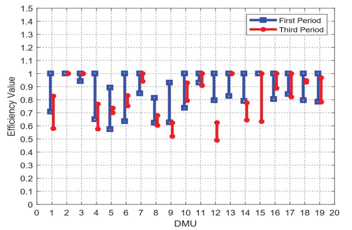
Interval efficiency of the first and third stages.
From the Figure 1, we can clearly see the overlapping and changing parts of the interval efficiency between the first and third stages. The elimination of environment variables and random errors,
At the same time, we rank the interval efficiency values of the third stage by taking the average of the upper and lower bounds of the interval as the criterion show in Table 5. The efficiency value by the traditional three-stage DEA model could be obtained from reference [34,43]. Comparing the ranking result with three-stage interval DEA model and the traditional three-stage DEA model in Table 6. By calculating the correlation coefficient, the fit of these two sets of rank results reaches 0.875. It shows that the overall trends of the two rank results are basically consistent.
| DMU | 1 | 2 | 3 | 4 | 5 | 6 | 7 | 8 | 9 | 10 | 11 | 12 | 13 | 14 | 15 | 16 | 17 | 18 | 19 |
|---|---|---|---|---|---|---|---|---|---|---|---|---|---|---|---|---|---|---|---|
| Traditional three-stage DEA model ranking | 16 | 1 | 1 | 15 | 7 | 8 | 1 | 14 | 18 | 9 | 1 | 19 | 5 | 17 | 13 | 11 | 12 | 6 | 10 |
| Three-stage interval DEA model ranking | 15 | 1 | 1 | 16 | 13 | 12 | 4 | 17 | 18 | 10 | 5 | 19 | 1 | 14 | 11 | 6 | 8 | 7 | 9 |
DEA, data envelopment analysis; DMU, decision-making unit.
Rank results of nineteen
4.2. Analysis of the Results for Identification of Benchmarks
Step 1: According to Eq. (14), the degree of efficiency change vector
| DMU | 1 | 2 | 3 | 4 | 5 | 6 | 7 | 8 | 9 | 10 |
|---|---|---|---|---|---|---|---|---|---|---|
| 0.818 | 1.000 | 1.062 | 0.883 | 1.216 | 1.183 | 1.108 | 0.967 | 0.828 | 1.076 | |
| 0.828 | 1.000 | 1.000 | 0.768 | 0.823 | 0.832 | 1.000 | 0.835 | 0.669 | 0.929 | |
| DMU | 11 | 12 | 13 | 14 | 15 | 16 | 17 | 18 | 19 | |
| 0.974 | 0.616 | 1.206 | 0.813 | 0.633 | 1.099 | 0.973 | 1.170 | 0.998 | ||
| 1.000 | 0625 | 1.000 | 0.777 | 1.000 | 1.000 | 1.000 | 0.947 | 0.965 | ||
DMU, decision-making unit.
The degree of efficiency change.
Step 2: According to the calculated vectors by Step 1 as elements, the system clustering is carried out according to the class average method, and the hierarchical diagram of the clustering results for nineteen
Step 3: It can be seen from Figure 2 that a total of five clusters are identified in this analysis. The best performing
The traditional improvement benchmark directly means that all noncompletely effective DMUs are improved according to the set of completely effective
4.3. Discussions
From the numerical examples, the main novelty and advantages of our proposed method are summarized as follows:
Hierarchical graph of clustering results.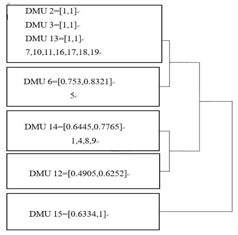
The proposed three-stage interval DEA model provides a novel way to deal with the interval input and output data. In the proposed method, the reasonable and effective way of coping with the effects of excluding external environmental factors and random errors is proposed. This is the distinct superiority and difference between the proposed method and other DEA models.
The improved benchmark is considered in the proposed method, its influence, and importance has been illustrated through the provided numerical examples. It can cluster DMUs which are naturally similar to provide improvement targets for poorly performing DMUs.
Like each coin has two sides, except for the aforementioned advantages, the proposed method has limitations in current version, i.e., it does not consider the preferences of decision makers during the decision process. Actually, the preferences are quite common in our daily life, which are practical and inevitable issues in the real-world situation, particularly under risk and uncertain environment. Although it is a limitation in the proposed method, it is one of the promising and solid future research directions, which can make the decision further close to the real-world situation.
5. CONCLUSIONS AND FUTURE WORKS
The traditional three-stage DEA model can evaluate the relative efficiency of a group of
In addition, from the perspective of environmental factors, this article combines the three-stage interval DEA model with clustering techniques to cluster naturally similar
Based on the analysis on this study, it is found that the proposed method not only improves the current studies, but also implies several promising and solid future research directions, i.e., (1) at present, only the case is considered where the input and output data is interval data. Where the environmental data is interval data, the case is worthy of our in-depth study. (2) This study considers the input–output indicators of
CONFLICT OF INTEREST
The authors declare no conflict of interest.
AUTHOR CONTRIBUTIONS
Guo-Qing Cheng: Conceptualization, Data curation, Formal analysis, Writing-original draft, Writing-review & editing. Liang Wang: Conceptualization, Data curation, Formal analysis, Writing-original draft, Writing-review & editing. Ying-Ming Wang: Conceptualization, Data curation, Formal analysis, Writing-original draft, Writing-review & editing.
ACKNOWLEDGMENTS
This work was partly supported by the National Natural Science Foundation of China (Project No. 71901071, 61773123).
REFERENCES
Cite this article
TY  - JOUR
AU  - Guo-Qing Cheng
AU  - Liang Wang
AU  - Ying-Ming Wang
PY  - 2020
DA  - 2020/10/29
TI  - An Extended Three-Stage DEA Model with Interval Inputs and Outputs
JO  - International Journal of Computational Intelligence Systems
SP  - 43
EP  - 53
VL  - 14
IS  - 1
SN  - 1875-6883
UR  - https://doi.org/10.2991/ijcis.d.201019.001
DO  - 10.2991/ijcis.d.201019.001
ID  - Cheng2020
ER  -