Uncertain Random Optimization Models Based on System Reliability

Qinqin Xu; Yuanguo Zhu

doi:10.2991/ijcis.d.200915.002

<Previous Article In Issue

Download article (PDF)

Next Article In Issue>

Volume 13, Issue 1, 2020, Pages 1498 - 1506

Uncertain Random Optimization Models Based on System Reliability

Authors

Qinqin Xu, Yuanguo Zhu^*^,

School of Science, Nanjing University of Science and Technology, Nanjing, Jiangsu, 210094, China

^*Corresponding author. Email: ygzhu@njust.edu.cn

Corresponding Author

Yuanguo Zhu

Received 1 May 2020, Accepted 8 September 2020, Available Online 24 September 2020.

DOI: 10.2991/ijcis.d.200915.002 How to use a DOI?
Keywords: Optimization model; Chance theory; Belief reliability; Hard failure; Soft failure; Jet pipe servo valve
Abstract: The reliability of a dynamic system is not constant under uncertain random environments due to the interaction of internal and external factors. The existing researches have shown that some complex systems may suffer from dependent failure processes which arising from hard failure and soft failure. In this paper, we will study the reliability of a dynamic system where the hard failure is caused by random shocks which are driven by a compound Poisson process, and soft failure occurs when total degradation processes, including uncertain degradation process and abrupt degradation shifts caused by shocks, reach a predetermined critical value. Two types of uncertain random optimization models are proposed to improve system reliability where belief reliability index is defined by chance distribution. Then the uncertain random optimization models are transformed into their equivalent deterministic forms on the basis of α-path, and the optimal solutions may be obtained with the aid of corresponding nonlinear optimization algorithms. A numerical example about a jet pipe servo valve is put forward to illustrate established models by numerical methods. The results indicate that the optimization models are effective to the reliability of engineering systems. It is our future work to consider an interdependent competing failure model where degradation processes and shocks can accelerate each other.
Copyright: © 2020 The Authors. Published by Atlantis Press B.V.
Open Access: This is an open access article distributed under the CC BY-NC 4.0 license (http://creativecommons.org/licenses/by-nc/4.0/).

1. INTRODUCTION

Reliability serves as one of vital essential characteristics of the system, which represents the capability of the system to carry out required functions. System reliability will be affected by several factors which can be divided into internal factors (wear, corrosion, fatigue, etc.) and external abrupt factors (impact, stress, etc.), which also known as degradation processes and shocks. Generally, the system failure caused by degradation processes is called soft failure. At a certain moment, the system suddenly fails due to accidental shocks, which is called hard failure.

In the traditional reliability assessment, a great quantity of literatures considered that the system failure is caused by soft failure or hard failure. Since 1990s, degradation process modeling has been used to analyze the reliability and statistical characteristics of the system [1–3]. There are also extensive researches on the modeling of shocks for the system suffered from hard failure [4–6]. However, most systems may be subject to hard failure and soft failure simultaneously due to exposure to degradation processes and external shocks. A system reliability model under the competing failure of extreme shock and internal degradation was proposed by Ye et al. [7]. Wang et al. [8] presented a competing failure model where the degradation rate is increased by shocks. Jiang et al. [9] proposed a reliability model for the systems subject to multiple s-dependent competing failure processes with a shifting failure threshold.

Scholars used to believe that only on the basis of enough failure data can we better select the reasonable metrics. However, traditional reliability assessment based on probability theory may be hindered by failure data which are difficult to acquire within a short time. Liu [10] pioneered uncertain reliability analysis of a dynamic system based on uncertainty theory with few failure data. Uncertainty theory associated with the experts' belief degrees was put forward by Liu [11] when there is no enough data to get a frequency distribution that an event will happen. Liu [12] also proposed the definition of uncertain process which is different from random process. Zeng et al. [13] put up reliability indexes which can evaluate product's reliability refer to uncertainty theory. Zeng et al. [14] also put up a minimal cut set-based numerical evaluation method to compute the system reliability index expressed by uncertain measure.

When there is a complicated system with a mixture of uncertainty and randomness, chance theory was put forward by Liu [15]. Liu [16] also proposed an optimization method to convert an uncertain random problem which is not easy to be solved into its deterministic form. After that, Wen and Kang [17] proposed a reliability assessment method in which reliability index was defined as chance distribution. Additionally, belief reliability metrics which are concerned with uncertain random variables were defined by Zhang et al. [18]. Some essential formulas were put forward by Gao and Yao [19] to calculate important indexes of common discrete uncertain random systems. Liu et al. [20] carried out the reliability analysis for uncertain random systems with independent degradation processes and shocks.

There are some research on the reliability optimization of uncertain random systems. Peng et al. [21] presented a new method to optimize the reliability of composite laminates taking into account uncertain parameters. A multi-objective optimization model to maximize the reliability of assembly line was proposed by Li et al. [22] under uncertain random environments. Optimization of maintenance policies which is severed as an critical role in reliability engineering has attracted much attention. Caballé et al. [23] proposed a preventive strategy applicable to the system based on reliability analysis. An optimal scheduling of inspection maintenance and replacement can optimize the system reliability considering the operational cost. Niwas and Garg [24] raised an approach to analyze system reliability and profit based on warranty policy. Chen and Li [25] determined an optimal replacement policy for minimizing the cost of the deteriorating system which is suffering random shocks and degradation processes. We will optimize the reliability of uncertain random systems motivated by these literature of system maintenance policy.

The system in this paper suffers from two dependent failure processes which may be modeled as uncertain degradation process and random shocks. The random shocks may also generate additional degradation shifts which may be driven by an uncertain renewal reward process. The competing failure models with extreme shock and cumulative shock are proposed respectively under uncertain random environment. This paper proposes a strategy of optimal allocation of maintenance resources to optimize the system reliability. The optimal maintenance strategy will be obtained to maximize the system reliability considering the different damage of degradation processes and shocks on system reliability. The system cost can also be saved by adjusting the proportion of maintenance resources.

The sections of this paper are listed below. Section 2 reviews some concepts involved in uncertainty theory. In Section 3, two types of uncertain random optimization system models are proposed, where reliability index is defined by chance distribution. The related algorithms of models are also discussed. In Section 4, the proposed models are verified by a numerical example. Section 5 summarizes this paper in a brief conclusion. Besides, for better comprehension of the article, some mathematical symbols used in the sequel are listed in the following notation.

Notation

H	Threshold value of soft failure
D	Threshold value of hard failure
λ	Intensity of shocks
N1(t)	Total shock times by time t
N2(t)	Total degradation shift times by time t
Zi	Magnitude of the i-th shock
	for i=1,2,⋯,N1(t)
F	Probability distribution of Zi
Yi	Magnitude of the i-th uncertain degradation
	shift for i=1,2,⋯,N2(t)
ηi	Interarrival time between i-th and i+1-th
	degradation shift for i=1,2,⋯,N2(t)
Xt	Degradation process
Wt	Wiener process
Ψ	Uncertainty distribution of ηi
ϒi	Uncertainty distribution of Yi
x0	Initial degradation value for the uncertain process
Re(u)	Reliability index of extreme shock model
Rc(u)	Reliability index of cumulative shock model

2. PRELIMINARY

Let Γ be a nonempty set, and ℒ be a σ-algebra over Γ. Each element Λ∈ℒ is called an event. A set function ℳ defined on the σ-algebra ℒ is called an uncertain measure [11] if it satisfies normality axiom, duality axiom, subadditivity axiom, and product axiom. An uncertain variable is a function ξ from an uncertainty space (Γ,ℒ,ℳ) to the set of real numbers such that the set {ξ∈B}={γ∈Γ∣ξ(γ)∈B} is an event for any Borel set of real numbers. The uncertainty distribution Φ(x):R→[0,1] of an uncertain variable ξ is defined as Φ(x)=ℳ{ξ≤x} for x∈R. An uncertain variable ξ is called normal if it has a normal uncertainty distribution

Φ(x)=1+expπ(e−x)3σ−1

denoted by N(e,σ) where e and σ are real numbers with σ>0. An uncertain variable ξ is called lognormal if lnξ is a normal uncertain variable N(e,σ).

Theorem 1.

(Liu [26]) Let Nt be a renewal process with i.i.d uncertain interarrival times {ξ1,ξ2,⋯}. If those interarrival times have a common uncertainty distribution Φ, then Nt has an uncertainty distribution

ϒt(x)=1−Φt∥x∥+1,∀x>0.(1)

Definition 1.

(Yao and Chen [27]) Let α be a number with 0<α<1. An uncertain differential equation dXt=f(t,Xt)dt+g(t,Xt)dCt is said to have an α-path Xtα (Ct is a Liu process) if it solves the corresponding ordinary differential equation dXtα=f(t,Xtα)dt+|g(t,Xtα)|Φ−1(α)dt, where Φ−1(α) is the inverse standard normal uncertain distribution, i.e.,

Φ−1(α)=3πlnα1−α.

Let (Γ,ℒ,ℳ) be an uncertainty space and (Ω,A,Pr) be a probability space. Then the product (Γ,ℒ,ℳ)×(Ω,A,Pr) is called a chance space. An uncertain random variable is a function ξ from a chance space (Γ,ℒ,ℳ)×(Ω,A,Pr) to the set of real numbers such that {ξ∈B} is an event for any Borel set B of real numbers. The chance measure of the uncertain random event {ξ∈B} is

Ch{ξ∈B}=∫01Pr{ω∈Ω|ℳ{γ∈Γ|ξ(γ,ω)∈B} ≥r}dr.

Theorem 2.

(Liu [15]) Let (Γ,ℒ,ℳ)×(Ω,A,Pr) be a chance space. Then

Ch{Λ×A}=ℳ{Λ}×Pr{A}

for any Λ∈ℒ and any A∈A.

3. SYSTEM RELIABILITY

Suppose that the system in this paper suffers from two dependent failures which are hard failure and soft failure, where either of failure processes can lead to system failures. Randomness and uncertainty exist simultaneously when analyzing the reliability of the system.

3.1. Hard Failure

Generally, a two-dimensional random vector sequence {(Ai,Zi)}i=0∞ has been used to describe the shock model. Assume Zi is the magnitude of the i-th shock, which represents the effect of the i-th shock on the system. {N1(t),t≥0} is the counting process generated by a sequence {Ai=0∞} in which Ai represents the interarrival time between two adjacent shocks.

Poisson process is a typical mathematical model of the counting process. Intuitively, the counting process of random events may be modeled as Poisson process as long as they occur independently in disjoint intervals and only once in sufficiently small intervals. External shocks approximately satisfy the above conditions in system reliability engineering. Thus, N1(t) may be regarded as a Poisson process to model total time of shocks. The nonnegative magnitudes of the i-th shock load are expressed as Zi which are i.i.d random variables.

3.1.1. Extreme shock model

In extreme shock model, the damage of shocks on the system is independent. Hard failure occurs when the size of any shock is beyond a specified threshold level D. The probability that no hard failure occurs by time t can be defined as

Pr⋂i=1N1(t)(h(u1,Zi)<D)(2)

where u1 is the control variable, h is a real function of u1 and Zi.

3.1.2. Cumulative shock model

It is assumed that the damage of shocks on the system is accumulated in cumulative shock model. The system will fail if the total magnitudes of accumulated shocks exceed a critical value D. The probability that there is no hard failure by time t can be described as

Pr∑i=1N1(t)h(u1,Zi)<D(3)

where u1 is the control variable, h is a real function of u1 and Zi.

Suppose h(u1,Zi) is a strictly monotone function with respect to Zi where u1 is the control variable, denoted as hu1(Zi).

3.2. Soft Failure

There is not enough failure data due to the limitation of time and cost in reliability assessment. Therefore, the traditional random process model is no longer applicable. The degradation may be evaluated by experts' experiment data based on uncertainty theory. Theoretically, it is appropriate to describe wear degradation with Liu process. The wear degradation Xt which can be modeled as

dXt=f(t,u2,Xt)dt+g(t,u2,Xt)dCt,(4)

where u2 is the control variable, Xt is the state variable (X0=x0), f and g are both real functions of time t, control variable u2, and state Xt, and Ct is Liu process.

It follows from Definition 1 that the solution Xt of (4) has an inverse uncertainty distribution

Φt−1(α)=Xtα(5)

where Xtα is the α-path.

The physical structure of the system may be damaged by external shock loads which can generate degradation shifts accumulated instantaneously when random shocks arrive. Since a large amount of data is not easy to derive in reliability assessment, it is more reasonable that degradation shifts are considered as an uncertain process.

Assume that the magnitude of the i-th uncertain degradation Yi are defined as i.i.d uncertain variables measured by experts' belief degrees. Here, the number of degradation shifts may be quantified by uncertain renewal process N2(t). The additional degradation shifts denoted as S(t) may be shown by uncertain renewal reward process

S(t)=∑i=1N2(t)Yi.(6)

Thus, the entire degradation is the sum of wear degradation process and degradation shifts. Soft failure occurs when the entire degradation processes reach a predetermined critical value H. The uncertain measure that there is no soft failure may be defined as

ℳXt+∑i=1N2(t)Yi<H.(7)

How to define a reliability index to measure reliability of complex systems is vital important in reliability engineering. Considering above two dependent failures, the reliability index may be regarded as belief reliability distribution. It is hopeful that uncertain degradation processes will not exceed the critical value H, and random shocks will not lead to system failures. The system can operate normally when neither failure process occurs.

Definition 2.

Assume that a system suffers from dependent soft failure and hard failure. Then the chance distribution of extreme shock model, i.e.,

ChXt+∑i=1N2(t)Yi<H,⋂i=1N1(t)(hu1(Zi)<D)(8)

is defined as belief reliability distribution Re(u).

Definition 3.

Assume that a system suffers from dependent soft failure and hard failure. Then the chance distribution of cumulative shock model, i.e.,

ChXt+∑i=1N2(t)Yi<H,∑i=1N1(t)hu1(Zi)<D(9)

is defined as belief reliability distribution Rc(u).

4. UNCERTAIN RANDOM OPTIMIZATION MODEL OF RELIABILITY

We are to optimize the reliability of a system by control variables which can be shown as regular inspections, maintenance funds, etc. Assume that u is a decision vector and R(u) (Re(u) or Rc(u)) is the objective function. Two optimization index models are presented with reference to the classification of shocks.

4.1. Optimization Model of Extreme Shock

In order to get the decision with the maximum reliability index satisfying a set of constraints, the maximum belief reliability index optimization model of extreme shock can be presented as

maxu1,u2∈UChXt+∑i=1N2(t)Yi<H,⋂i=1N1(t)(hu1(Zi)<D)subject todXt=f(t,u2,Xt)dt+g(t,u2,Xt)dCtg(u1,u2)≤0X0=x0.(10)

It is a nature approach to transform the model (10) to an equivalent problem which may be easy to be solved.

Remark 2.

Compared with existing uncertain random systems in [15,16,28], the reliability index in proposed models is also defined by chance distribution. For the continuous system subject to competing failure processes, the models in [17] suffer from the independent degradation process and shocks. In contrast, the advantages of our model in this paper are mainly reflected in the following:

The system failure is subject to dependent competing failure processes which are uncertain wear degradation process and random shocks;
The dependence of the wear degradation process and shocks is that random shocks may accelerate wear degradation process by degradation shifts which are driven by an uncertain renewal reward process;
The proposed uncertain random constrained model may be transformed into a nonlinear constrained programming problem by uncertainty theory;
The system reliability is optimized by optimal allocation ratio of maintenance resources considering the different damage of degradation processes and shocks on system reliability.

Theorem 3.

Let Xt be a wear degradation process, N1(t) be a Poisson process with intensity λ, and Zi be i.i.d shock loads with probability distribution F. Assume i.i.d interarrival times ηi and independent shock damages Yi are uncertain variables whose uncertainty distributions are Ψ and ϒi, respectively. Then the optimization model of extreme shock (10) is equivalent to following form:

maxu1,u2∈U1−Ψ(t)∧J1(H)∨(maxm≥1(1−Ψ(t1+m))∧J2(H))×exp(−λt)(1+∑m=1∞(λt)mm!(L(hu1−1(D)))m)subject todXtα=f(t,u2,Xtα)dt+|g(t,u2,Xtα)|Φ−1(α)dtg(u1,u2)≤0X0=x0,(11)

where L(hu1−1(D)) is

L(hu1−1(D))=F(hu1−1(D)),if hu1(z)is a strictly increasingfunction with respect to z1−F(hu1−1(D)),if hu1(z)is a strictly decreasingfunction with respect to z

J1(H) is the root α of the equation

Xtα−H=0,

and J2(H) is the root α of the equation

Xtα+∑i=1kϒi−1(α)−H=0.

Proof

Obviously, Xt+∑i=1N2(t)Yi<H is an uncertain event, and ⋂i=1N1(t)(hu1(Zi)<D) is a random event. It follows from Theorem 2 immediately that the chance measure is the product of uncertain measure and probability measure,

ChXt+∑i=1N2(t)Yi<H,⋂i=1N1(t)(hu1(Zi)<D)= ℳXt+∑i=1N2(t)Yi<H×Pr⋂i=1N1(t)(hu1(Zi)<D).

Part I: Since the degradation shifts follow from an uncertain renewal reward process, we can get

ℳXt+∑i=1N2(t)Yi<H =ℳ⋃m=0∞(N2(t)=m)∩Xt+∑i=1mYi<H =ℳ⋃m=0∞(N2(t)≤m)∩Xt+∑i=1mYi<H =ℳ(N2(t)≤0)∩(Xt<H) ∨maxm≥1ℳ(N2(t)≤m)∩Xt+∑i=1mYi<H =(ℳ{N2(t)≤0}∧ℳ{Xt<H}) ∨maxm≥1ℳ{N2(t)≤m}∧ℳXt+∑i=1mYi<H

On the one hand, the uncertain distribution of N2(t) can be calculated by Eq. (1)

ℳ{N2(t)≤0}=1−Ψ(t),ℳ{N2(t)≤m}=1−Ψt1+m.

One the other hand, it follows from (5) that Xt has an inverse uncertainty distribution Xtα. Write J1(H)=ℳ{Xt<H}=α∈(0,1). That is, J1(H) is the root α of the equation

Xtα−H=0.

Referring to operational laws of uncertain variables, the inverse uncertainty distribution of ∑i=1mYi can be computed by ∑i=1mϒi−1(α). Write J2(H)=ℳ{Xt+∑i=1mYi<H}=α∈(0,1). That is, J2(H) is the root α of equation

∑i=1mϒi−1(α)+Xtα−H=0.

We have

ℳXt+∑i=1N2(t)Yi<H =(1−Ψ(t)∧J1(H))∨maxm≥11−Ψt1+m ∧J2(H).

Part II: The random shock follows from the compound Poisson process, we can obtain

Pr⋂i=1N1(t)(hu1(Zi)<D) =Pr⋃m=0∞(N1(t)=m)∩⋂i=1m(hu1(Zi)<D) =Pr{N1(t)=0} +∑m=1∞Pr(N1(t)=m)∩⋂i=1m(hu1(Zi)<D) =Pr{N1(t)=0} +∑m=1∞Pr{N1(t)=m}Pr⋂i=1m(hu1(Zi)<D)

Since N1(t) is a Poisson process with intensity λ, then

Pr{N1(t)=0}=exp(−λt) Pr{N1(t)=m}=exp(−λt)(λt)mm!.

As mentioned above, hu1(Zi) is a monotone function with respect to Zi. When hu1(Zi) is a strictly increasing function, we have

L(hu1−1(D))=Pr{hu1(Zi)≤D} =Pr{Zi≤hu1−1(D)}=F(hu1−1(D)).

When hu1(Zi) is a strictly decreasing function, then

L(hu1−1(D))=Pr{hu1(Zi)≤D} =Pr{Zi≥hu1−1(D)}=1−F(hu1−1(D)).

And then

∏i=1mPr{hu1(Zi)<D}=(L(hu1−1(D)))m.

Thus we can derive

Pr⋂i=1N1(t)(hu1(Zi)<D)=exp(−λt)1+∑m=1∞(λt)mm!(L(hu1−1(D)))m,

the theorem is verified.

4.2. Algorithm for Extreme Shock Optimization Model

The optimization model with extreme shock may be converted into it's equivalent problem by Theorem 3, then the problem becomes a typical nonlinear constrained programming problem. The penalty function algorithm with conjugate gradient method for nonlinear programming problems with inequality constraints is adopted in this section.

Algorithm 1:

Penalty function algorithm for (11)

Fix a time t and set X0=x0,k=0,l=0,M0>0,c≥2, ε>0 (a predetermined precision).
Construct a new function Q(u,Ml)=R(u)+MlG(g(u)) where G(g(u))=[max{0,g(u)}]2.
For initial value uk=(u1k,u2k), set β=0, γ=1, and α=(β+γ)∕2. Then solve the corresponding differential equations
dXtα=f(t,u2k,Xtα)dt +g(t,u2k,Xtα)Φ−1(α)dt
by Euler method.
If Xtα−HXtγ−H≤0, then set β=α. Otherwise, set γ=α.
If γ−β>ε, set α=(γ+β)∕2 and go to step 4. Otherwise, output α as the root J1(H).
Compute J2(H) similarly to the steps 3 – 5. Then set hk=∇Q(uk,Ml), pk=−hk.
Compute the step length λk by the line search Q(uk+λkpk,Ml)=maxλ>0Q(uk+λpk,Ml). Then set uk+1=uk+λkpk.
k=k+1,hk=∇Q(uk,Ml).
If ∥hk∥≤ε, go to step 13, otherwise, perform the next step.
If k=n, go to step 12. Otherwise, perform the next step.
Compute pk=−hk+∥hk∥2∥hk−1∥2pk−1 and go to step 7.
Carry out a new round of iteration from uk, go to step 3.
If MlG(g(uk))≤ε, then u∗=uk is the optimal solution. The algorithm ends. Otherwise, Ml+1=cMl, l=l+1, go to step 2.

4.3. Optimization Model of Cumulative Shock

Referring to extreme shock optimization model, we are to present a maximum reliability index optimization model with cumulative shock which can be described as

maxu1,u2∈UChXt+∑i=1N2(t)Yi<H,∑i=1N1(t)hu1(Zi)<Dsubject todXt=f(t,u2,Xt)dt+g(t,u2,Xt)dCtg(u1,u2)≤0X0=x0.(12)

Theorem 4.

Let Xt be a wear degradation process, N1(t) be a Poisson process with intensity λ and Zi be i.i.d shock loads with probability distribution F. Assume i.i.d interarrival times ηi and independent shock damages Yi are uncertain variables whose uncertainty distributions are Ψ and ϒi, respectively. The optimization model of cumulative shock (12) can be converted into their corresponding deterministic form

maxu1,u2∈U1−Ψ(t)∧J1(H)∨(maxm≥1(1−Ψ(t1+m))∧J2(H))×exp(−λt)(1+∑m=1∞(λt)mm!Lhu1(D)∗)subject todXtα=f(t,u2,Xtα)dt+|g(t,u2,Xtα)|Φ−1(α)dtg(u1,u2)≤0X0=x0(13)

where Lhu1(D)∗ is the m-convolution

Lhu1(D)∗=L(hu1(z))∗⋯∗L(hu1(z))|z=D,

L(hu1−1(D))=F(hu1−1(D)),if hu1(z)is a strictly increasingfunction with respect to z1−F(hu1−1(D)),if hu1(z)is a strictly decreasingfunction with respect to z

J1(H) is the root α of the equation

Xtα−H=0,

and J2(H) is the root α of the equation

Xtα+∑i=1kϒi−1(α)−H=0.

Proof

The proof is similar to that of Theorem 3.

4.4. Algorithm for Cumulative Shock Optimization Model

Algorithm 1 may be utilized to obtain the optimal solutions of cumulative shock optimization problem. The difference between two models (11) and (13) is that they have different terms L(hu1−1(D)) and Lhu1(D)∗ in the objective functions. Thus, a key point applying Algorithm 1 to problem (13) is to calculate m-convolution Lhu1(D)∗ by Monte Carlo simulation (Algorithm 2).

Algorithm 2:

Monte Carlo simulation for m-convolution

Set the initial value k=0, i=1, N>0, m>0 and D>0.
Generate numbers h1,h2,⋯,hm randomly with distribution L(hu1(z)) for each u1.
Compute Si by Si=h1+h2+⋯+hm.
If Si<D, k=k+1.
i=i+1.
If i=N, output the value k∕N as Lhu1(D)∗ and stop. Otherwise, go to step 2.

5. NUMERICAL EXPERIMENT

The jet pipe servo valve is a representative two-stage electro hydraulic flow valve of EHSVs in modern industrial control systems, which can realize the servo control of mechanical equipments. In the following, we will analyze and optimize the reliability of jet pipe servo valve based on proposed models.

5.1. Proposed Model Description

The study indicates that the main cause of system failures is the fluid deterioration which would cause clamping stagnation and tribological wear between the spool and the sleeve. The clamping stagnation can cause additional wear debris, which would both affect the reliability of the system.

The clamping stagnation is considered as hard failure which is driven by a compound Poisson process with intensity λ. We assume that magnitude of the i-th clamping stagnation Zi are i.i.d normal random variables, the magnitude of the i-th additional wear debris Yi are i.i.d normal uncertain variables, the interarrival time between i-th and i+1-th wear debris ηi are i.i.d lognormal uncertain variables. Since the degradation processes of the system usually follows the law of exponential decay. It is assumed that shock rate and wear rate which are generated by maintenance funds exhibit an exponential decay function. Thus, suppose that u1 is the proportion of maintenance funds on clamping stagnation that yields the shock rate e−u1. Then

h(u1,Zi)=e−u1Zi.

The tribological wear is driven by an uncertain process

dXt=ae−u2dt+be−u2dCt,

where a is the drift coefficient, b is the diffusion coefficient, u2 is the proportion of maintenance funds on tribological wear, and e−u2 is the wear rate. The relevant parameters are shown in Table 1.

Parameters	Values	Sources
H	5 mm	[30]
D	40 N	[30]
λ	2.5×10−5	[30]
Z	Z∼N(30,52)N	[30]
η	η∼ℒOGN(3.4×104,102) h	Assumption
Y	Y∼N(0.4,0.12) mm	Assumption
Ỹ	Y∼N(0.5,0.12) mm	[30]
a	10−3	Assumption
b	2×10−3	Assumption
x0	0	[30]

Table 1

Parameter values.

5.2. Traditional Model Description

The traditional reliability evaluation is modeled based on probability theory in which all the variables Yĩ involved are random variables, and the degradation process is driven by random process. The tribological wear can be described as

dXt=adt+bdWt

where Wt is a standard Wiener process. Referring to [29], we can get the evaluation method of system reliability. The relevant parameters are displayed in Table 1. Next, the numerical results of proposed uncertain random system reliability model would be compared with traditional reliability model.

Remark 2.

In the numerical experiments, we choose the mostly common probability distribution functions which conform to the physical characteristics of the system according to the reference [30]. The uncertain distribution functions are given based on the experience of experts. Of course, other continuous distribution functions may also be applied. Since the model proposed in this paper is continuous, we have not adopted the discrete distribution function for the time being. In the future, we will carry out the reliability optimization of discrete-time systems to further improve the research of system reliability.

5.3. Results and Analysis Figure 1

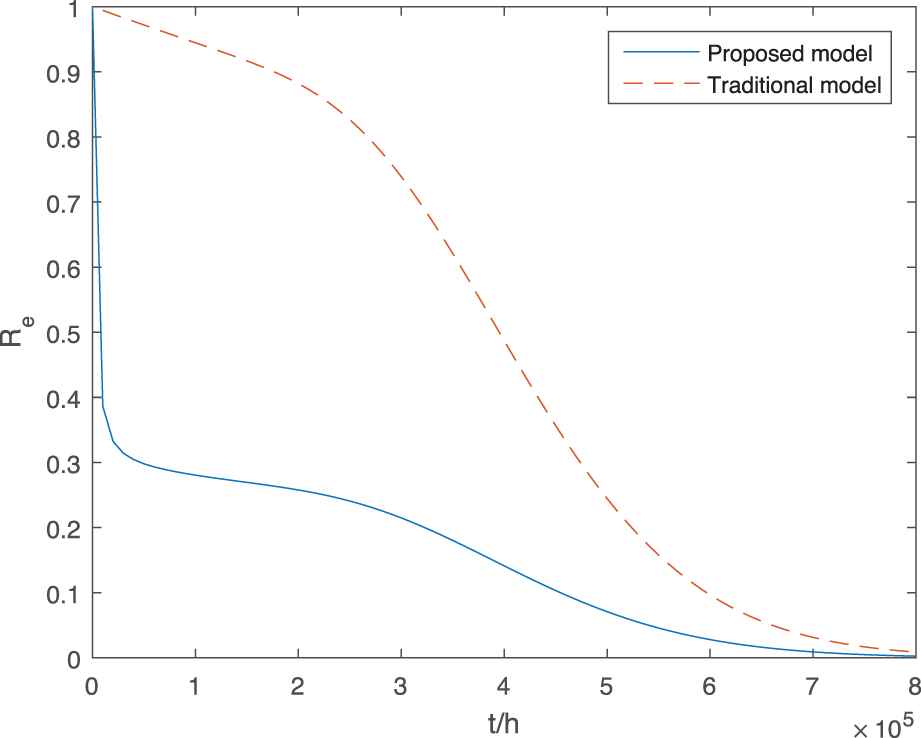
In Figure 1, Re represents the original reliability index with extreme shock of two models. The numerical result shows that the reliability index of traditional model is always more than that of the proposed model. The reliability index decreases gradually with time t, which conforms to the failure process of extreme shock model.

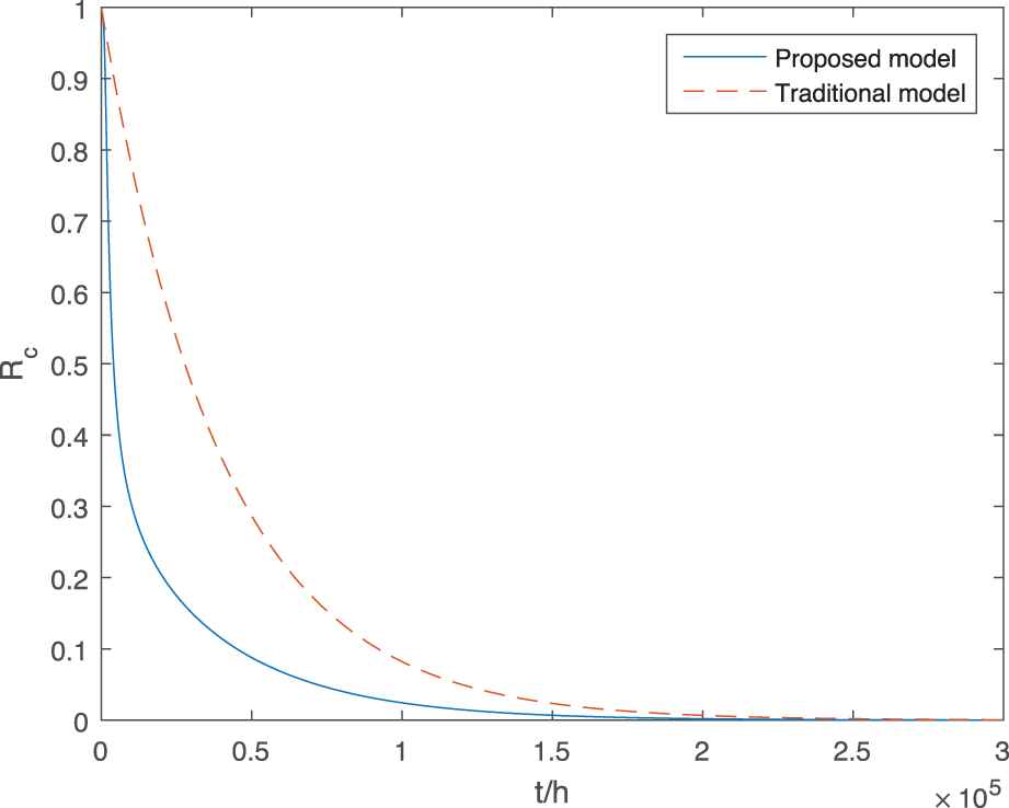
In Figure 2, Rc represents the original reliability index with cumulative shock of two models. Similarly, the reliability of the traditional random model is higher than that of the uncertain random model. The reliability of the system decreases with time t, which accords with the physical characteristics of system reliability.

The experimental data show that evaluation models proposed in this paper are relatively conservative when traditional evaluation models tend to overestimate the system reliability. The internal degradation that may not be quantified as random events due to the lack of failure data, while we may regard them as uncertain events according to experts' experience. If the degradation processes are regarded as random events, the reliability of the system will be overestimated, which will lead to the wrong configuration of maintenance strategy, causing system failure, greatly shortening the system life, and causing economic losses.

The two uncertain random optimization models have been transformed into the nonlinear constrained programming problems by Theorems 3 and 4, respectively. There are lots of software that may be used to solve such typical optimization problems. In this paper, the mathematical software MATLAB is selected to obtain the optimal solutions based on above algorithms.

Then, we select 10 sets of data from optimization model proposed to compare and illustrate the optimization decisions. In Table 2, Re(u∗) is the optimal reliability index of extreme shock optimization model with optimal control variables u∗ obtained by Algorithm 1. In Table 3, Rc(u∗) is the optimal reliability index of cumulative shock optimization model with optimal control variables u∗ obtained by Algorithms 1 and 2. Re(u) and Rc(u) are the original reliability indexes of two models without control variables, respectively.

t(h)	u∗	Re(u∗)	Re
1×103	(0.6355,0.3607)	0.9963	0.9736
2×103	(0.6109,0.3881)	0.9195	0.7949
3×103	(0.5763,0.4226)	0.8021	0.6456
4×103	(0.5524,0.4473)	0.7040	0.5552
5×103	(0.5209,0.4762)	0.6349	0.4986
6×103	(0.5038,0.4951)	0.5825	0.4607
7×103	(0.4893,0.5106)	0.5430	0.4339
8×103	(0.4655,0.5328)	0.5147	0.4139
9×103	(0.4312,0.5574)	0.4932	0.3985
10×103	(0.4153,0.5844)	0.4767	0.3863

Table 2

Optimal solutions and original index of extreme shock model.

t(h)	u∗	Rc(u∗)	Rc
1×103	(0.7426,0.2544)	0.9684	0.9501
2×103	(0.7135,0.2863)	0.8486	0.7570
3×103	(0.6472,0.3528)	0.7202	0.6000
4×103	(0.6157,0.3274)	0.5977	0.5035
5×103	(0.5842,0.3619)	0.5274	0.4412
6×103	(0.5436,0.4246)	0.4836	0.3979
7×103	(0.5079,0.4635)	0.4455	0.3657
8×103	(0.4318,0.5226)	0.4194	0.3404
9×103	(0.4005,0.5735)	0.3967	0.3199
10×103	(0.3628,0.6247)	0.3777	0.3026

Table 3

Optimal solutions and original index of cumulative shock model.

From these 10 sets of data, we may see that the reliability of the system decreases with time t. In addition, the reliability decay rate of our optimization model is relatively slow. This means that a reasonable proportion of maintenance allocation can slow down the rate of reliability decline when considering degradation and external shocks.

It can also be easily observed that the optimal reliability indexes of two models are always greater than their original indexes when time t varies from 103 to 10×103, which indicate that the uncertain random optimization models are effective and practical in reliability engineering.

The data also show that the maintain fund on tribological wear is increasing when time t varies from 103 to 10×103. An explanation for this phenomenon is that clamping stagnation will generate abrupt wear debris. The particle wear always exists in EHSV's working, while clamping stagnation is an abrupt failure. Soft failure caused by tribological wear gradually turns into the main failure behavior with the increase of system operation time. The wear debris increasingly to the critical value should require more funds as time goes on.

We may conclude that optimal maintenance allocation can improve the system reliability and delay the decay rate of system reliability from the above numerical experimental results. In addition, it may be seen from the optimal solutions that the clamping stagnation is the main failure process in initial time of system operation. And with the gradual accumulation of wear debris, tribological wear becomes the main failure process of the system. This shows that the damage of clamping stagnation and tribological wear on system reliability is variable in different periods. Thus, it is necessary to adjust the proportion of maintenance allocation to maximize the system reliability.

6. CONCLUSION

In this paper, we present a type of shock-degradation dependence of the uncertain random system where random shocks can accelerate wear degradation process by additional degradation shifts. The wear degradation process is driven by an uncertain process, random shocks are driven by a compound Poisson process, degradation shifts are modeled as an uncertain renew reward process. Then, two optimization reliability index models are introduced and algorithms of models are also proposed. Finally, a numerical example about a jet pipe servo valve is given to illustrate the obtained results. Furthermore, the existing research can be extended to an interdependent competing failure model where the degradation processes and shocks can accelerate each other.

CONFLICTS OF INTEREST

The authors declare they have no conflicts of interest.

AUTHORS' CONTRIBUTIONS

All authors have the same contributions to prepare the manuscript.

ACKNOWLEDGMENTS

This work is supported by the National Natural Science Foundation of China (Grant No. 61673011).

REFERENCES

1.C. Lu and W. Meeker, Using degradation measures to estimate a time-to-failure distribution, Technometrics, Vol. 35, 1993, pp. 161-174.

2.N. Singpurwalla, Survival in Dynamic Environments, Reliability and Risk: a Bayesian Perspective, John Wiley & Sons, Ltd., New York, USA, 1995.

3.J. Kharoufeh and S. Cos, Stochastic models for degradation-based reliability, IIE Trans., Vol. 37, 2005, pp. 533-542.

4.T. Nakagawa, Shock and Damage Models in Reliability Theory, Springer, London, England, 2007.

5.Y. Chien, S. Sheu, Z. Zhang, et al., An extended optimal replacement model of systems subject to shocks, Eur. J. Oper. Res., Vol. 175, 2006, pp. 399-412.

6.J. Bai, Z. Li, and X. Kong, Generalized shock models based on a cluster point process, IEEE Trans. Reliab., Vol. 55, 2006, pp. 542-550.

7.Z. Ye, L. Tang, and H. Xu, A distribution-based systems reliability model under extreme shocks and natural degradation, IEEE Trans. Reliab., Vol. 60, 2011, pp. 246-256.

8.Z. Wang, H. Huang, and Y. Li, An approach to reliability assessment under degradation and shock process, IEEE Trans. Reliab., Vol. 60, 2011, pp. 852-863.

9.L. Jiang, Q. Feng, and D. Coit, Reliability and maintenance modeling for dependent competing failure processes with shifting failure thresholds, IEEE Trans. Reliab., Vol. 61, 2012, pp. 932-948.

10.B. Liu, Uncertain risk analysis and uncertain reliability analysis, J. Uncertain Syst., Vol. 4, 2010, pp. 163-170.

11.B. Liu, Uncertainty Theory, second, Springer-Verlag, Berlin, Germany, 2007.

12.B. Liu, Fuzzy process, hybrid process and uncertain process, J. Uncertain Syst., Vol. 2, 2008, pp. 3-16.

13.Z. Zeng, M. Wen, and R. Kang, Belief reliability: a new metrics for products' reliability, Fuzzy Optim. Decis. Making, Vol. 12, 2013, pp. 15-27.

14.Z. Zeng, R. Kang, M. Wen, et al., Uncertainty theory as a basis for belief reliability, Inf. Sci., Vol. 429, 2018, pp. 26-36.

15.Y. Liu, Uncertain random variables: a mixture of uncertainty and randomness, Soft Comput., Vol. 17, 2013, pp. 625-634.

16.Y. Liu, Uncertain random programming with applications, Fuzzy Optim. Decis. Making, Vol. 12, 2013, pp. 153-169.

17.M. Wen and R. Kang, Reliability analysis in uncertain random system, Fuzzy Optim. Decis. Making, Vol. 15, 2016, pp. 491-506.

18.Q. Zhang, R. Kang, and M. Wen, Belief reliability for uncertain random systems, IEEE Trans. Fuzzy Syst., Vol. 26, 2018, pp. 3605-3614.

19.R. Gao and K. Yao, Importance index of components in uncertain random systems, Knowl. Based Syst., Vol. 109, 2016, pp. 208-217.

20.B. Liu, Z. Zhang, and Y. Wen, Reliability analysis for devices subject to competing failure processes based on chance theory, Appl. Math. Model., Vol. 75, 2019, pp. 398-413.

21.X. Peng, Y. Guo, C. Qiu, et al., Reliability optimization design for composite laminated plate considering multiple types of uncertain parameters, Eng. Optim., 2020.

22.Y. Li, R. Peng, I. Kucukkoc, et al., System reliability optimization for an assembly line under uncertain random environment, Comput. Ind. Eng., Vol. 146, 2020, pp. 106-118.

23.N. Caballé, I. Castro, C. Pérez, et al., A condition-based maintenance of a dependent degradation-threshold-shock model in a system with multiple degradation processes, Reliab. Eng. Syst. Safety, Vol. 134, 2015, pp. 98-109.

24.R. Niwas and H. Garg, An approach for analyzing the reliability and profit of an industrial system based on the cost free warranty policy, J. Braz. Soc. Mech. Sci. Eng., Vol. 40, 2018, pp. 265.

25.J. Chen and Z. Li, An extended extreme shock maintenance model for a deteriorating system, Reliab. Eng. Syst. Safety, Vol. 93, 2017, pp. 1123-1129.

26.B. Liu, Uncertainty Theory: a Branch of Mathematics for Modeling Human Uncertainty, Springer-Verlag, Berlin, Germany, 2010.

27.K. Yao and X. Chen, A numerical method for solving uncertain differential equations, J. Intell. Fuzzy Syst., Vol. 25, 2013, pp. 825-832.

28.T. Zu, R. Kang, M. Wen, et al., Belief reliability distribution based on maximum entropy orinciple, IEEE Access, Vol. 6, 2018, pp. 1577-1582.

29.H. Peng, Q. Feng, and D. Coit, Reliability and maintenance modeling for systems subject to multiple dependent competing failure processes, IIE Trans., Vol. 43, 2010, pp. 12-22.

30.H. Che, S. Zeng, and J. Guo, Reliability modeling for dependent competing failure processes with mutually dependent degradation process and shock process, Reliab. Eng. Syst. Safety, Vol. 180, 2018, pp. 168-178.

<Previous Article In Issue

Download article (PDF)

Next Article In Issue>

Journal: International Journal of Computational Intelligence Systems
Volume-Issue: 13 - 1
Pages: 1498 - 1506
Publication Date: 2020/09/24
ISSN (Online): 1875-6883
ISSN (Print): 1875-6891
DOI: 10.2991/ijcis.d.200915.002 How to use a DOI?
Open Access: This is an open access article distributed under the CC BY-NC 4.0 license (http://creativecommons.org/licenses/by-nc/4.0/).

Cite this article

ris enw bib

TY  - JOUR
AU  - Qinqin Xu
AU  - Yuanguo Zhu
PY  - 2020
DA  - 2020/09/24
TI  - Uncertain Random Optimization Models Based on System Reliability
JO  - International Journal of Computational Intelligence Systems
SP  - 1498
EP  - 1506
VL  - 13
IS  - 1
SN  - 1875-6883
UR  - https://doi.org/10.2991/ijcis.d.200915.002
DO  - 10.2991/ijcis.d.200915.002
ID  - Xu2020
ER  -

download .riscopy to clipboard