
Attribute Reduction of Boolean Matrix in Neighborhood Rough Set Model

- DOI
- 10.2991/ijcis.d.200915.004How to use a DOI?
- Keywords
- Neighborhood rough set; Boolean matrix; Attribute reduction; GPU
- Abstract
Neighborhood rough set is a powerful tool to deal with continuous value information systems. Graphics processing unit (GPU) computing can efficiently accelerate the calculation of the attribute reduction and approximation sets based on matrix. In this paper, we rewrite neighborhood approximation sets in the matrix-based form. Based on the matrix-based neighborhood approximation sets, we propose the relative dependency degree of attributes and the corresponding algorithm (DBM). Furthermore, we design the reduction algorithm (ARNI) for continuous value information systems. Compared with other algorithms, ARNI can effectively remove redundant attributes, and less affect the classification accuracy. On the other hand, the experiment shows ARNI based on the matrixing rough set model can significantly speed up by GPU. The speedup is many times over the central processing unit implementation.
- Copyright
- © 2020 The Authors. Published by Atlantis Press B.V.
- Open Access
- This is an open access article distributed under the CC BY-NC 4.0 license (http://creativecommons.org/licenses/by-nc/4.0/).
1. INTRODUCTION
The explosive growth of data volume increases the complexity of data, and makes data processing more difficult than before. By reducing unnecessary or irrelevant attributes in the data, the efficiency of decision-making can be improved. The rough set theory proposed by Pawlak can quickly deal with uncertain and inaccurate problems [1], which has been widely used in machine learning, data mining, and other fields [2]. To construct an equivalence relation of Pawlak rough set for continuous value information system, the continuous values need to be clustered into some mutually disjoint blocks. However, discretizing the continuous values exists some uncertainty and may lose some essential information. To solve this problem, many rough set models have been proposed, such as fuzzy rough sets [3–6], covering rough sets [7–9], semi-monolayer cover rough set [10], neighborhood rough sets [11–14], granule-based rough sets [15–17]. Neighborhood rough set is a feasible model to handle continuous values without discretization.
In neighborhood rough sets, the calculation, whether two elements are neighborhoods or not, becomes easier and more localized compared to other methods [11]. It offers better potential for parallel and distributed computation [18]. Furthermore, by marking the neighborhood of the element, we can label some data to improve the usability for lack-of-label big data [19]. However, the complexity of the calculation is an unavoidable question on neighborhood rough set [19,20].
Matrix description makes the calculation of approximation sets more efficient. Huang et al. [21] defined three composition operations, and studied their characteristic matrices, and investigated the relationship between the characteristic matrices and covering approximation operators. Wang et al. [22] represented three types of existing covering approximation operators with the Boolean matrix. Ma [23] selected more covering approximation model and rewrote them in a high level.
Graphics processing unit (GPU) acceleration is widely used not only in deep learning [24] but also in the operations of the dense matrices and blocks [25], such as minimizing the encountered in the transformation of tensor contractions into matrix multiplications [26], object sorting [27], computation of equivalence classes, and approximation sets [28]. Generally, GPU is at least 10 times faster than the coetaneous central processing unit (CPU) [29]. Zhang et al. [30] adopted a multi-GPU solution to accelerate their algorithm about a parallel method for computing approximations based on matrix and achieved 334.9 times of acceleration compared to the CPU.
The matrixing of the whole computation process is the premise of the speedup by GPU. For neighborhood rough approximation operators, the relation of disjunction and conjunction among Boolean matrices can represent the relation of union and intersection between sets. Through a sequence of substitution operations, the operation of the neighborhood rough set will be transformed from element-based form to matrix-based form. Furthermore, we proposed the relative dependency degree of attributes based on matrixing neighborhood approximation sets, and the corresponding reduction algorithms (DBM and ARNI).
This paper is organized as follows: In Section 2, some basic concepts about neighborhood rough sets are introduced. In Section 3, we propose attribute reduction algorithms DBM and ARNI based on the Boolean matrix. In Section 4, a series of comparative experiments are designed to show the feasibility and efficiency of ARNI. Section 5 is the conclusion of this paper.
2. PRELIMINARIES
In information systems, the elements can easily cluster into some information granules by different methods. How to describe them systematically in a framework is a basic question about the construction of approximation space in rough set theory. The binary relation and neighborhood system are two common entry points. Binary relation can summarize the principle of generating information granules. Covering or neighborhood systems directly organize the related elements into a block or a neighborhood. In classic Pawlak rough set, the equivalence relation and equivalence classes can transform mutually. However, in other models, the transformation is no longer smooth [31]. The choice binary relation orneighborhood system depends almost entirely on the character in information systems. For example, in set-valued or incomplete information systems, we can use not only tolerance relation and its generalized tolerance relation [18] but also maximal consistent blocks [11] or semi-monolayer covering [10] to organize the blocks on the system. For the information system with noise, the variable precision binary relation [32] and probabilistic binary relation [33] are frequently mentioned. For continuous information systems, we can build a hypersphere neighborhood to describe a similar degree among the elements, as shown in Figure 1.
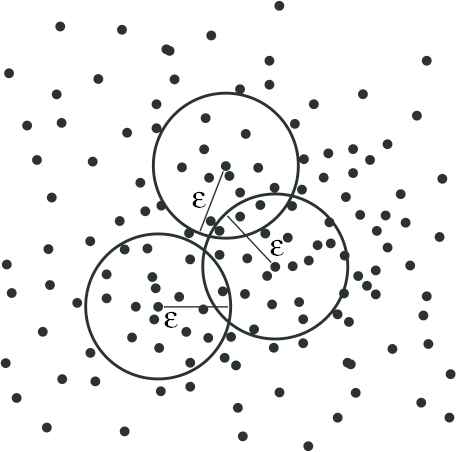
Neighborhood of the elements
In this section, we introduce the basic concepts about neighborhood rough set and two Boolean matrix operations.
2.1. Neighborhood Rough Set
In information systems, let
Definition 1.
[12,13] In the neighborhood system
Hu proposed the definition of the neighborhood rough sets [13,14], which is a specialized covering rough model in neighborhood approximation space (Definition 2).
Definition 2.
[11–14,34] In the neighborhood system
Example 1.
Given a neighborhood decision system
| U | a1 | a2 | a3 | a4 | d |
|---|---|---|---|---|---|
| x1 | 0.9 | 0.6 | 1.4 | 1.3 | 0 |
| x2 | 0.5 | 1.0 | 1.5 | 1.1 | 0 |
| x3 | 0.6 | 1.3 | 1.4 | 1.0 | 1 |
| x4 | 1.0 | 1.2 | 1.7 | 1.5 | 1 |
| x5 | 1.1 | 0.9 | 2.5 | 1.4 | 1 |
Decision information system.
The values of neighborhoods are
By (2) and (3), the upper and lower approximation sets of the neighborhood rough set are as follows:
2.2. Boolean Matrix Operation
Boolean matrix has been used to describe the classic binary relation or neighborhood system frequently. To matrix the upper and lower neighborhood approximation operations, we need to upgrade some operations based on traditional disjunction and conjunction to calculate the union and intersection of two sets.
Definition 3.
[23,34] Let
3. ATTRIBUTE REDUCTION BASED ON BOOLEAN MATRIX
In this section, Boolean matrix operations (
3.1. Boolean Matrix Representation of Approximations
In this section, we rewrite the neighborhood approximation operation by the Boolean matrix and its matrix operations.
Definition 5.
[34] In the neighborhood system
Obviously, this definition indicates that
For any
Definition 6.
[22,23] In the approximation space
Proposition 1.
In the neighborhood approximation space
Proof
(
(
Thus,
The proof of formula (10) is similar to that of formula (9), then proposition 1 is held.
Definition 7.
[34] In the neighborhood approximation space
Definition 8.
In the neighborhood approximation space
Suppose that eigenvectors
So far, we have accomplished the matrix description of the neighborhood rough set.
Example 2 (Continuing Example 1).
Let
The relation matrix
The upper and lower approximation sets of
Similarly,
By the matrixing method, we still get the same result as Example 1.
3.2. Reduction of Neighborhood Rough Set
Dependency and importance degree are widely used in attribute reduction. For neighborhood rough set, we specified the two indexes based on the approximation sets.
Definition 9.
In neighborhood approximation space
Unless particularly stated, the relative dependency degree is the dependency degree of the decision-making
Definition 10.
[34,35] In the neighborhood decision system
If
If
Definition 11.
In the neighborhood decision system
Example 3 (Continuing Example 2).
Let
The eigenvector corresponding to the upper and lower approximations of
Thus, the dependency degree of
Similarly, the dependency degrees of other condition attributes are shown in Table 2. Because
The result of the subset of condition-attribute sets.
3.3. Attribute Reduction Algorithm Based on Boolean Matrix
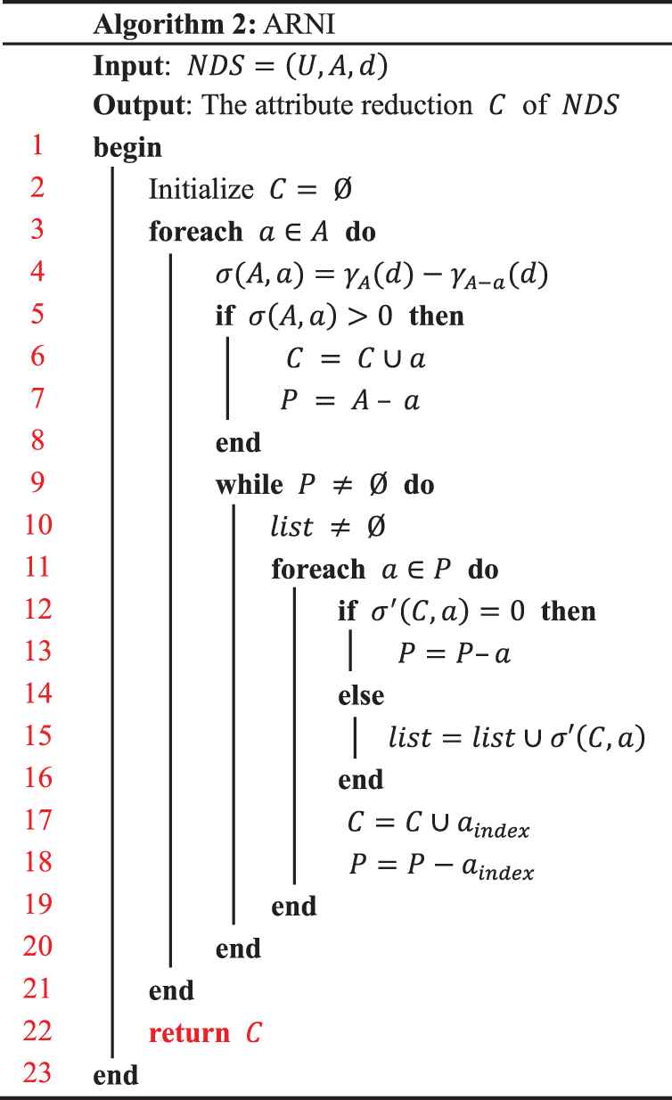
Based on the previous propositions and definitions, we design two algorithms Dependency Degree based on Boolean Matrix (DBM) and Attribute Reduction based on Neighborhood Importance Degree (ARNI).
Algorithm DBM is used to calculate the dependency degree of the condition attribute with respect to decision attributes in the data set. Suppose that there are
ARNI calls DBM to calculate the neighborhood importance degree of
4. EXPERIMENTS
In the experiment, we use Algorithm DBM to calculate the relative dependency degree for every condition attribute. In Algorithm ARNI, the redundant attributes will be reduced from the continuous information systems. To verify the feasibility and effectiveness of ARNI, we design a series of comparative experiments. Specifically, we divide the experiments into two parts. One part is the reduction ability of the algorithm ARNI. In another part, we test the acceleration performance of GPU for the matrixing models.
4.1. Experiment Environment and Objects
The experimental data in this paper come from the UCI machine learning database [36], which is listed in Table 3. All values in those datasets will be normalized before we used.
| Data Sets | Logogram | Samples | Attributes | Classes |
|---|---|---|---|---|
| biodeg | BI | 1055 | 41 | 2 |
| debrecen | DR | 1151 | 19 | 2 |
| ForestTypes | FT | 326 | 27 | 4 |
| glass | GL | 214 | 10 | 6 |
| ionosphere | IP | 351 | 33 | 2 |
| iris | IR | 150 | 4 | 3 |
| movement_libras | ML | 360 | 90 | 15 |
| sonar | SN | 208 | 60 | 2 |
| wdbc | WD | 569 | 30 | 2 |
| wine | WI | 178 | 13 | 9 |
Description of data sets.
Algorithms DBM and ARNI are programmed in Python 3.6.7. The experiments run on a computer with Windows 7 Ultimate, Intel i5-5200U CPU 2.2GHz, and 4GB memory, NVIDIA 820M.
4.2. Comparative Experiment between ARNI and Other Reduction Algorithms
To demonstrate the effectiveness of ARNI, we compare our algorithm with NRS, CRS, and PCA in terms of the classification performance of K-Nearest Neighbor, K = 3 (KNN) and Support Vector Machine (SVM).

NRS is another classic reduction algorithm in neighborhood rough set theory [12,13]. Table 4 shows the number of features after reduction by ARNI and NRS for the different radius of the hypersphere neighborhood
| ε | NRS |
ARNI |
|||||
|---|---|---|---|---|---|---|---|
| Data Sets | Reduction |
Accuracy |
Reduction |
Accuracy |
|||
| KNN | SVM | KNN | SVM | ||||
| 0.01 | BI | 9 | 0.8216 | 0.7128 | 9 | 0.8216 | 0.7128 |
| DR | 7 | 0.6221 | 0.5951 | 8 | 0.6413 | 0.6245 | |
| FT | 4 | 0.8108 | 0.7293 | 6 | 0.8234 | 0.7183 | |
| GL | 4 | 0.6889 | 0.5653 | 4 | 0.6889 | 0.5653 | |
| IP | 5 | 0.9007 | 0.8638 | 5 | 0.9007 | 0.8638 | |
| IR | 3 | 0.9533 | 0.9667 | 3 | 0.9533 | 0.9667 | |
| ML | 7 | 0.5956 | 0.3980 | 12 | 0.6811 | 0.4235 | |
| SN | 4 | 0.5889 | 0.5374 | 7 | 0.6218 | 0.6134 | |
| WD | 4 | 0.8999 | 0.9177 | 6 | 0.9189 | 0.9255 | |
| WI | 4 | 0.8144 | 0.8147 | 6 | 0.95131 | 0.96663 | |
| 0.05 | BI | 14 | 0.8284 | 0.6948 | 13 | 0.8328 | 0.7493 |
| DR | 13 | 0.6230 | 0.6168 | 11 | 0.6334 | 0.6213 | |
| FT | 7 | 0.8393 | 0.7414 | 9 | 0.8306 | 0.7298 | |
| GL | 9 | 0.6555 | 0.4696 | 8 | 0.6641 | 0.4958 | |
| IP | 6 | 0.9091 | 0.8867 | 6 | 0.9091 | 0.8867 | |
| IR | 3 | 0.9533 | 0.9667 | 3 | 0.9533 | 0.9667 | |
| ML | 31 | 0.7011 | 0.4111 | 22 | 0.6989 | 0.4564 | |
| SN | 7 | 0.5794 | 0.5753 | 11 | 0.6375 | 0.6384 | |
| WD | 9 | 0.9316 | 0.9230 | 10 | 0.9489 | 0.9216 | |
| WI | 5 | 0.8262 | 0.8141 | 4 | 0.8783 | 0.8818 | |
| 0.1 | BI | 23 | 0.8159 | 0.7658 | 20 | 0.8200 | 0.7625 |
| DR | 19 | 0.6229 | 0.6142 | 17 | 0.6213 | 0.6169 | |
| FT | 17 | 0.8429 | 0.7379 | 19 | 0.8436 | 0.7379 | |
| GL | 9 | 0.6555 | 0.4696 | 7 | 0.6479 | 0.4563 | |
| IP | 8 | 0.8952 | 0.8780 | 8 | 0.8952 | 0.8780 | |
| IR | 4 | 0.9533 | 0.9667 | 3 | 0.9533 | 0.9667 | |
| ML | 23 | 0.7000 | 0.4089 | 19 | 0.7167 | 0.4360 | |
| SN | 9 | 0.6493 | 0.6492 | 11 | 0.6375 | 0.6384 | |
| WD | 11 | 0.9403 | 0.9213 | 11 | 0.9403 | 0.9213 | |
| WI | 6 | 0.8655 | 0.8655 | 4 | 0.8783 | 0.8818 | |
ARNI, Attribute Reduction based on Neighborhood Importance Degree; KNN, K-nearest neighbor; SVM, support vector machine.
Reduction results of two different algorithms.
Next, we provide a comprehensive comparison of the effects of ARNI, NRS, and other reduction algorithms based on non-neighborhood rough set theory. Those algorithms include the reduction algorithm classic rough set (CRS) [1] and principal component analysis (PCA) in the number of attributes and classification accuracy after reduction. For ARNI and NRS, we choose a moderate-performance parameter
The results of the comparative experiment are shown in Table 5. The classifiers perform better in the ARNI reduced decision systems than other algorithms. That is to say, the reduction of attributes based on ARNI provided better support for KNN and SVM than others.
| RAW |
CRS |
NRS |
PCA |
ARNI |
|||||||||||
|---|---|---|---|---|---|---|---|---|---|---|---|---|---|---|---|
| Data Sets | Reduction | KNN | SVM | Reduction | KNN | SVM | Reduction | KNN | SVM | Reduction | KNN | SVM | Reduction | KNN | SVM |
| BI | 41 | 0.8368 | 0.7725 | 33 | 0.8368 | 0.7772 | 9 | 0.8216 | 0.7128 | 9 | 0.8226 | 0.7008 | 9 | 0.8216 | 0.7128 |
| DR | 19 | 0.6229 | 0.6142 | 17 | 0.6203 | 0.6142 | 7 | 0.6221 | 0.5951 | 8 | 0.6117 | 0.6156 | 8 | 0.6413 | 0.6245 |
| FT | 27 | 0.8168 | 0.7042 | 18 | 0.7908 | 0.6374 | 4 | 0.8108 | 0.7293 | 6 | 0.8025 | 0.7178 | 6 | 0.8234 | 0.7183 |
| GL | 10 | 0.6555 | 0.4696 | 8 | 0.6379 | 0.4973 | 4 | 0.6889 | 0.5653 | 4 | 0.6690 | 0.5277 | 4 | 0.6889 | 0.5653 |
| IP | 33 | 0.8553 | 0.8523 | 27 | 0.8437 | 0.8664 | 5 | 0.9007 | 0.8638 | 5 | 0.8693 | 0.8809 | 5 | 0.9007 | 0.8638 |
| IR | 4 | 0.9533 | 0.9667 | 4 | 0.9533 | 0.9667 | 3 | 0.9533 | 0.9667 | 3 | 0.9533 | 0.9600 | 3 | 0.9533 | 0.9667 |
| ML | 90 | 0.7956 | 0.5389 | 17 | 0.7389 | 0.4678 | 7 | 0.5956 | 0.3980 | 12 | 0.6900 | 0.5889 | 12 | 0.6811 | 0.4235 |
| SN | 60 | 0.6432 | 0.6388 | 9 | 0.6498 | 0.7024 | 4 | 0.5889 | 0.5374 | 7 | 0.6644 | 0.6726 | 7 | 0.6722 | 0.6134 |
| WD | 30 | 0.9702 | 0.9527 | 23 | 0.9648 | 0.9474 | 4 | 0.8999 | 0.9177 | 6 | 0.9499 | 0.9422 | 6 | 0.9189 | 0.9255 |
| WI | 13 | 0.9555 | 0.9781 | 13 | 0.9555 | 0.9781 | 4 | 0.8144 | 0.8147 | 6 | 0.9513 | 0.9666 | 6 | 0.9513 | 0.9667 |
ARNI, Attribute Reduction based on Neighborhood Importance Degree; KNN, K-nearest neighbor; SVM, support vector machine; CRS, classic rough set; PCA, principal component analysis.
Reduction results of different algorithms.
4.3. Experiment about the Effect of ε
The granularity
The range of
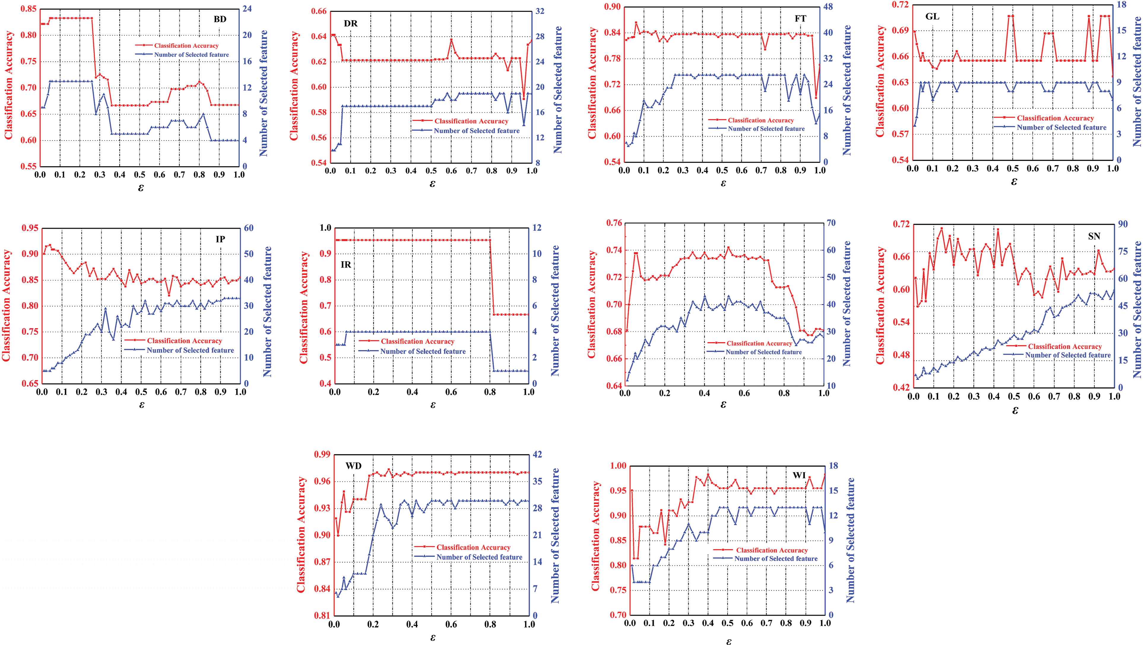
Numbers of selected features and classification accuracy with the different granularity
4.4. Experiment about GPU Acceleration
GPU architecture consists of a set of streaming multiprocessors (SMs), each of which contains a set of processor cores called streaming processors (SPs). Therefore, multiple threads are suitable for a large number of repeated or parallel operations. Using GPU acceleration operations can effectively improve computational efficiency.
Compute Unified Device Architecture (CUDA), introduced by NVIDIA, is a heterogeneous parallel computing model that involves both CPU and GPU. In this paper, we use CUDA V7.0 [37] and Pytorch framework [38] to recode ARNI in it. The program runs on CPU versus GPU. The acceleration times are shown in Figure 3. The speedup ratio
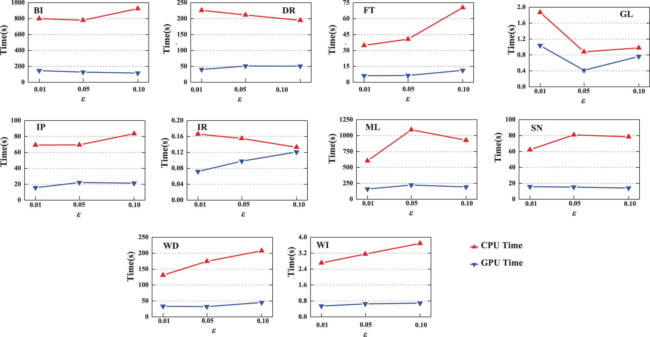
Running time on using only central processing unit (CPU) and using graphics processing unit (GPU) acceleration with different data sets.
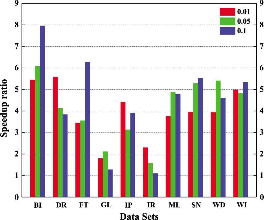
Speedup ratio of graphics processing unit (GPU) with different datasets.
5. CONCLUSION
It is a core challenge to the rough set theory about how to reduce attributes effectively in information systems. The matrix description of rough sets and reduction algorithm can be executed more efficiently than other forms in the computer operation, especially in GPU. In this paper, we propose an attribute reduction algorithm for neighborhood rough set based on Boolean matrix. Specifically, we define the dependency degree of decision attribute sets. Based on matrix description of neighborhood rough set, we also give a solving method for the relative dependency degree by matrix computing (Algorithm DBM). Furthermore, we realized the attribute reduction by matrix computing (Algorithm ARNI). The results in UCI datasets show that comparing the existing attribute reduction algorithms ARNI can reduce attributes less affecting the classification accuracy. Besides, we also show the acceleration performance of GPU for the matrixing model.
CONFLICT OF INTEREST
The authors declare that there is no conflict of interest.
AUTHORS’ CONTRIBUTIONS
Yan Gao conceived and designed the study. Changwei Lv performed the experiments and wrote the paper. Zhengjiang Wu reviewed and edited the manuscript. All authors read and approved the manuscript.
ACKNOWLEDGMENTS
This work was supported by the National Natural Science Foundation of China (No. 11601129, 61972134).
REFERENCES
Cite this article
TY  - JOUR
AU  - Yan Gao
AU  - Changwei Lv
AU  - Zhengjiang Wu
PY  - 2020
DA  - 2020/09/21
TI  - Attribute Reduction of Boolean Matrix in Neighborhood Rough Set Model
JO  - International Journal of Computational Intelligence Systems
SP  - 1473
EP  - 1482
VL  - 13
IS  - 1
SN  - 1875-6883
UR  - https://doi.org/10.2991/ijcis.d.200915.004
DO  - 10.2991/ijcis.d.200915.004
ID  - Gao2020
ER  -