
A Novel Particle Swarm Optimization Approach to Support Decision-Making in the Multi-Round of an Auction by Game Theory
 , Xuan-Thang Nguyen1, , Gia Nhu Nguyen3, 4, , Dac-Nhuong Le4, 5, 6, *,
 - DOI
- 10.2991/ijcis.d.200828.002How to use a DOI?
- Keywords
- Multi-round procurement; Project conflicts; Game theory; Particle swarm optimization; Nash equilibrium; Decision support system; Multi-objective
- Abstract
In this paper, game-theoretic optimization by particle swarm optimization (PSO) is used to determine the Nash equilibrium value, in order to resolve the confusion in choosing appropriate bidders in multi-round procurement. To this end, we introduce an approach that proposes (i) a game-theoretic model of the multi-round procurement problem; (ii) a Nash equilibrium strategy corresponding to the multi-round strategy bid; and (iii) an application of PSO for the determination of the global Nash equilibrium point. The balance point in Nash equilibrium can help to maintain a sustainable structure, not only in terms of project management but also in terms of future cooperation. As an alternative to procuring entities subjectively, a methodology using Nash equilibrium to support decision-making is developed to create a balance point that benefits procurement in which buyers and suppliers need multiple rounds of bidding. To solve complex optimization problems like this, PSO has been found to be one of the most effective meta-heuristic algorithms. These results propose a sustainable optimization procedure for the question of how to choose bidders and ensure a win-win relationship for all participants involved in the multi-round procurement process.
- Copyright
- © 2020 The Authors. Published by Atlantis Press B.V.
- Open Access
- This is an open access article distributed under the CC BY-NC 4.0 license (http://creativecommons.org/licenses/by-nc/4.0/).
1. INTRODUCTION
Project management is a key activity in software development organizations. One of the key problems in software project planning is the scheduling, which involves resource allocation and scheduling activities on time, optimizing the cost and/or duration of the project. The scheduling is a complex constrained optimization problem, because for the optimization of resources, time, and cost, it is necessary to consider a combination of variables, rules, and restrictions that cause the problem to be NP-hard search-based software engineering (SBSE) is an emerging area focused on solving software engineering problems by using search-based optimization algorithms. SBSE has been applied to several problems which arise during the software life cycle. The software project scheduling problem (SPSP) consists in finding a suitable assignment of employees to tasks, such that the project can be delivered in the shortest possible time and with the minimum cost [1,2].
In recent years, a considerable amount of research has been conducted around this topic. The studies that have been performed have focused on different aspects, for instance, on proposing models to solve the problem of allocating employees to tasks so that the project’s cost and duration are minimized, on introducing or applying more efficient optimization algorithms, and on studying the performance of different metaheuristics to determine which may be more appropriate to solve the problem.
We summarize generalizations of the activity concept, the precedence relations and of the resource constraints. Alternative objectives and approaches for scheduling multiple projects are discussed as well. In addition to popular variants and extensions such as multiple modes, minimal and maximal time lags, and net present value-based objectives in Table 1 [1–6].
| Problem | Types | Ref |
|---|---|---|
| Project Scheduling Problem (PSP) | Single-objective | [1,2] |
| Project Scheduling Problem Work-Content (PSPWC) | Single-objective | [1] |
| Resource-Un-Constrained Project Scheduling Problem (RUCPSP) | Multi-objectives | [1] |
| Software Project Scheduling Problem (SPSP) | Multi-objectives | [3] |
| Resource Constrained Projects (RCP) | Multi-objectives | [2] |
| Resource Constrained Project Scheduling Problem (RCPSP) | Multi-objectives | [2] |
| Preemptive-Resource Constrained Project Scheduling Problem (P-RCPSP) | Multi-objectives | [1] |
| Resource-Constrained Project Scheduling Problem with Minimal and Maximal Time Lags (RCPSP/max) | Multi-objectives | [2] |
| Resource-Constrained Project Scheduling Problem with Flexible Work Profile (RCPSP-FW) | Multi-objectives | [1] |
| Flexible-Resource Constrained Project Scheduling Problem (F-RCPSP) | Multi-objectives | [1] |
| Preemptive-Flexible-Resource-Constrained Project Scheduling Problem (P-F-RCPSP) | Multi-objectives | [1] |
| Resource Constrained Multi-Project Scheduling Problem (RCMPSP) | Multi-objectives | [4] |
| Preemptive-Resource Constrained Multi-Project Scheduling Problem (P-RCMPSP) | Multi-objectives | [1] |
| P-RCMPSP with permitted Mode Change (P-MRCPSP-MC) | Multi-objectives | [1] |
| Flexible-Resource Constrained Multi-Project Scheduling Problem (F-RCMPSP) | Multi-objectives | [1] |
| Resource Availability Cost Problem (RACP) | Multi-objectives | [2] |
| Resource-Constrained Project Scheduling Problem with Generalized Precedence (RCPSP-GPR) | Multi-objectives | [4] |
| Resource constrained project scheduling problem with cash flows (RCPSPCF) | Multi-objectives | [3] |
| Multi-Mode Resource Constrained Project Scheduling Problem (MRCPSP) | Multi-objectives | [2] |
| Preemptive-Flexible-Resource-Constrained Multi-Project Scheduling Problem (P-F-RCMPSP) | Multi-objectives | [1] |
| Multi-Mode Resource Constrained Project Scheduling Problem with Renewable Resource (MRCPSP-RR) | Multi-objectives | [1] |
| Preemptive-Multi-mode Resource-constrained Project Scheduling Problem (P-MRCPSP) | Multi-objectives | [1] |
| MRCPSP Problem with Minimal and Maximal Time Lags (MRCPSP/max) | Multi-objectives | [2] |
| Resource-constrained project scheduling problem with time-dependent resource capacities | Multi-objectives | [2] |
| Resource Investment Problem with Minimal and Maximal Time Lags (RIP/max) | Multi-objectives | [2] |
| Search-based Software Engineering (SBSE) | Single-objective | [1] |
| Work Breakdown Schedule (WBS) | Multi-objectives | [4] |
| Team Software Project Management Problem (TSPMP) | Multi-objectives | [5] |
The software project management problems.
As we can see in Table 1, the RCPSP can be classified by preemptive scheduling, resource requests varying with time, setup times, multiple modes, tradeoff problems, minimal time lags, maximal time lags, release dates and deadlines, time-switch constraints, etc. The RCPSP is a general problem in scheduling that has a wide variety of applications in manufacturing, production planning, project management, and various other areas. In this study, we aim to identify the key aspects of procurement in the software project management context and their relation to project success [2].
Project management is the core process of most current business activities, which include projects that have the goal of creating products, services, or original results. Project management tasks include project scope management, quality, project schedule, budget, resources, and risks. Still, there are more internal problems affecting the project which is out of the management of risk management parts such as the conflicts between the project partners or the conflicts in risk management itself. Therefore, detecting and analyzing these problems brings a necessary supplement for the project management tasks, thus ensuring all matters arising to be controlled and also enhancing the quality and chances of success of the project [1,2]. Based on various factors such as the source, cause, role, or function of conflicts in the project, conflicts can be classified into several categories as follows:
By source of conflict, conflicts are classified as (i) conflict from plan scheduling, (ii) conflict from determining the priority in performing project task, (iii) conflict from the power sources, (iv) conflict from technical problems, (v) conflict from administrative procedure, (vi) conflict from the private issue, and (vii) conflict from the expenditure.
By cause of conflict, conflicts are classified as (i) conflict from different goals, (ii) conflict from resource disparity, (iii) conflict by other people’s obstruction, (iv) conflict due to stress and psychological pressure from many people, (v) conflict due to ambiguity of jurisdiction, and (vi) conflict due to misleading communication.
By role, conflicts are classified as (i) positive conflict and (ii) negative conflict.
By function, conflicts are classified as (i) functional conflict and (ii) dysfunctional conflict.
Procurement is viewed as a strategic function to improve an organization’s profitability. In recent years, it has been shown that there are many challenges and difficulties in procurement, especially in multi-round procurement, where the result of selecting bidders in one round affects bidding behavior in subsequent rounds [7].
The first challenge is the difficulty in choosing the right bidders to maximize profits while also ensuring project completion, which becomes more and more challenging when it is divided into many stages with several auction-goers. The material depends on each company and their pricing policies, which must be considered in order to choose the most reasonable ones (Quality and Cost-based Selection). However, quality cannot be assured afterward [8]. This implies many risks, as there are no measures or evidence to prove that the chosen bidder is the best one. Moreover, a win-win relationship requires a fair auctioning environment, which is ideal when all bidders are granted the highest profits.
Secondly, dividing the project into many stages affects the project’s total cost, which is related to time. Good sustainability strategies require lowering the cost and, hence, increasing the profits and reducing the predicted price of each package; otherwise, it can lead to package over-budget, which causes incompletion and risks for the project.
In summary, a scientific and applicable method is necessary to make the final decision of the auction [8–13]. Apart from that, the main questions which must be considered for the problem are as follows:
When is the best time to open a bid?
Who are the most suitable auction-goers?
What are the most suitable quality and price at each stage?
How can we solve this?
The term sustainability strategy can be explained as a prioritized set of actions which provides an agreed framework in a cooperation situation. In other words, there are countless benefits from a good sustainability strategy, in terms of cooperation in a project, making the jobs of participants easier because long-term cooperation can be maintained by a rational plan of action. Rationality makes sustainability more effective and easier when it comes to project integration. Rationality can be obtained by forming a win-win situation for all sides.
Despite the fact that, in some special types of problems, Nash equilibrium may not perform as well as other models, such as competitive equilibrium (i.e., when dividing the channels into two categories: high-quality and low-quality), it is still the most suitable model to find the appropriate benefit for all players by determining a win-win relationship [14–17].
The multi-round procurement problem was being an NP-hard problem, solution methods are primarily meta-heuristics. The above questions have already been answered by some researchers using genetic algorithms (GAs) and the Nash equilibrium [14,18]. However, when the threshold is changed, the performance of each algorithm is different.
Particle swarm optimization (PSO) and evolutionary algorithms such as GA have been used to solve multi-objective problems; they have many similar behaviors but also have differences in performance across certain problem areas. They both have the same mechanism, in that the system is initialized by generating a population randomly and searching for optima by refining this population. Nonetheless, PSO does not use techniques such as cross-over and mutation for updating and, so, may prematurely converge to a local optimum. The authors prove that PSO and GA have the same effectiveness in solution quality, but that PSO has superior computational efficiency over GA. The advantages of PSO are that it uses fewer parameters and evaluation functions than GA [19].
The main idea of GA is combining father and mother singles to generate many descendants, in order to create a better generation. In contrast, the PSO Algorithm focuses on developing its own members to better themselves. Therefore, instead of using GA and generating 100 particles, we can use PSO with fewer individuals and let them improve themselves [20,21]. For these reasons, we propose a new approach using PSO and Nash equilibrium to identify a sustainability strategy in a multi-round procurement problem which has higher accuracy and better speed. The following sections explain further details about the problem under consideration.
Our main contributions is presented a novel approach for solving a multi-round procurement. In this approach, by combining knowledge from the fields of game theory, Nash equilibrium, and PSO algorithm, we presented a game theory model as an optimal cooperative solution for the multi-round procurement problem. The parameter setting strategy is selected in an attempt to fine-tune the PSO algorithm for this problem. The Nash equilibrium point can be considered as the best solution for the conflict. The Nash equilibrium point can be solved by multi-objectives evolutionary algorithm. Compared with another multi-objectives evolutionary algorithms, the result suggested that PSO algorithm was significantly better than others with shorter runtime and higher quality for finding Nash equilibrium candidate in large-scale dataset.
2. RELATED WORKS
The software project management was being an NP-hard problem, solution methods are primarily meta-heuristics. We classify and present the state-of-the-art hybrid meta-heuristics for software project management and multi-round procurement problems in Table 2 [20–29]. These methods can be categorized based on local search meta-heuristics, evolutionary and population-based, learning meta-heuristics, and our proposed algorithms
| Classes of Algorithms | Authors | Year | Ref |
|---|---|---|---|
| 1. Local Search Meta-heuristics Algorithms | |||
| HL (Hill Climbing) | Kolisch et al. | 1999 | [24] |
| TB (Tabu search with Path Re-linking Strategy) | Nonobe and Ibaraki | 2002 | [25] |
| GRASP (Greedy randomized adaptive search procedure) | Kochetov and Stolyar | 2003 | [25] |
| LNS (Large Neighborhood Search) | Palpant et al. | 2004 | [26] |
| SA (Simulated Annealing) | Mika et al. | 2005 | [27] |
| SS (Scatter Search and Electromagnetism Theory) | Debels et al. | 2006 | [24] |
| RS (Random Search) | Chen et al. | 2009 | [25] |
| ALNS (Adaptive Large Neighborhood Search) | Muller L.F | 2009 | [24] |
| FAF (Filter-and-Fan) | He et al. | 2016 | [28] |
| 2. Evolutionary and Population-based Algorithms | |||
| GDE3 (3rd Evolution Step of Generalized DE) | Kukkonen and Lampinen | 2005 | [29] |
| AGA (Adaptive Genetic Algorithm) | Kim et al. | 2006 | [30] |
| CGA (Competent Genetic Algorithm) | Yassine et al. | 2007 | [28] |
| GA (Genetic Algorithm) | Chang et al. | 2008 | [27] |
| GP (Genetic Programming)/GALib | Chang et al. | 2008 | [31] |
| SMPSO (Speed-Constrained Multi-objective PSO) | Nebro et al. | 2008 | [28] |
| MOCell (Multi-Objective Cellular Genetic) | Nebro et al. | 2009 | [28] |
| MOFA (Multi-Omics Factor Analysis) | Yang | 2009 | [28] |
| Li and Zhang | 2009 | [32] | |
| DEA (Differential Evolution Algorithm) | Wu et al. | 2010 | [28] |
| Vanucci et al. | 2012 | [33] | |
| NSGA II (Adaptive |
Deb et al. | 2012 | [33] |
| MOGA (Multi-Objective Genetic Algorithm) | Stylianou et al. | 2013 | [34] |
| NSGA (Non-Dominated Sorting Genetic Algorithm) | Amiri et al. | 2013 | [33] |
| PAES (Pareto Archived Evolution Strategy) | Wang et al. | 2013 | [27] |
| DEPT (Differential Evolution) | Chen and Ni | 2014 | [28] |
| NSGA-III (Non-Dominated Sorting Genetic Algorithm III) | Mkaouer et al. | 2015 | [35] |
| SPEA2 (Strength Pareto Evolutionary Algorithm 2) | Deb et al. | 2015 | [36] |
| MOEA (Multi-Objective Evolutionary Algorithm) | Hadka | 2015 | [34] |
| NSGA-II |
Myszkowski et al. | 2017 | [37] |
| NSGA-II |
Gholizadeh and Afshar | 2018 | [37] |
| AI (Artificial Immune) | Agarwal et al. | 2007 | [20] |
| EOD (Estimation of Distribution) | Fang et al. | 2010 | [20] |
| SFL (Shuffle Frog-Leaping) | Fang and Wang | 2012 | [20] |
| FA (Firefly Algorithm) | Sanaei et al. | 2013 | [27] |
| MA (Memetic Algorithm) | Wang and Liu | 2013 | [28] |
| GE (Grammatical Evolution) | Barros et al. | 2013 | [28] |
| PSO (Particle Swarm Optimization) | Zeighami et al. | 2013 | [27] |
| BCO (Bee Colony Optimization) | Nouri et al. | 2013 | [27] |
| ACO (Ant Colony Optimization) | Xiao et al. | 2013 | [25] |
| PBIL (Population-Based Incremental Learning) | Jin et al. | 2014 | [28] |
| IWD (Intelligent Water Drops) | Crawford et al. | 2018 | [28] |
| MOABC (Multi-Objective Artificial Bee Colony) | Gong et al. | 2018 | [28] |
| 3. Hybrids Meta-heuristics Algorithms | |||
| ANGEL (Integrating ACO, GA and Local Search) | Tseng and Chen | 2006 | [38] |
| HEA (Hybrid Evolutionary Algorithm) | Rogalska et al. | 2008 | [39] |
| (1+1) EA and RS (Evolutionary Algorithm with Random Search) | Yannibelli and Amandi | 2013 | [40] |
| EHH (Evolutionary Hyper-Heuristic) | Wu et al. | 2016 | [41] |
| Tree search + GA | Zamani | 2017 | [42] |
| Hybrid ABC-PSO | Khuat et al. | 2018 | [43] |
| 4. Learning and Parallel Metaheuristics Algorithms | |||
| PL (Population Learning) | Jedrzejowicz et al. | 2006 | [44] |
| NN (Neural network) | Jaberi and Jaberi | 2014 | [45] |
| PPSO (PSO Parallel) | Fahmy et al. | 2014 | [46] |
| Tabu Search Parallel | Bukata et al. | 2015 | [47] |
| PACO (ACO Parallel) | Thiruvady et al. | 2019 | [48] |
| 5. Our algorithms proposed | |||
| GANE (Genetic Algorithm and Nash Equilibrium) | Trinh Ngoc Bao et al. | 2017 | [49] |
| BCPM (Bayesian Critical Path Method) | Nguyen Ngoc Tuan et al. | 2018 | [50] |
| UGM (Unified Game-Based Model) | Trinh Ngoc Bao et al. | 2019 | [51] |
| NAM (Nash Equilibrium Model) | Quyet-Thang Huynh et al. | 2019 | [52] |
| Probabilistic Method | Quyet-Thang Huynh et al. | 2020 | [53] |
| MMAS (Min-Max Ant System) | Dac-Nhuong Le et al. | 2020 | [54] |
Summary of the classification algorithms for the software project management and multi-round procurement problems.
In [12], the authors designed a new approach to find a winner in a multiple-attribute auction. The new method could help to address a mechanism for decision-making in dealing with multiple-attribute and multiple-sourcing procurement. Multiple-sourcing is usually proposed to prevent a variety of procurement risk and uncertainty. In [22], a model was developed to assist participants in multiple-attribute procurement in inferring their preference, based on the difficulty of elicitation.
In [23], the ability to use Bayesian equilibrium to predict human behavior in sealed-bid split-award procurement auctions was analyzed. The auction type was a multi-object extension, in which bidders may require more than one unit. The authors applied the Bayes–Nash equilibrium in the expanded game to forecast the strategies of participants. Then, they experimented with the accuracy of the equilibrium with computerized bidders. The results showed that the complexity of the multi-object does not have much effect on the result of procurement; rather, the risk aversion has a more pronounced effect.
In game theory, Nash equilibrium has been used to analyze the outcome of strategic interaction and also how conflict may be mitigated in competitive environments. A Nash solution is a mixed strategy profile with the property that no single player can obtain a higher value of expected utility by deviating unilaterally from this profile. It means all players obtain more revenue under cooperation, and thereby promoting sustainability. The above questions are already answered by some researchers using the GA and the Nash equilibrium. However, when the number of a threshold is changed, the performance of each algorithm is different. Furthermore, there are many meta-heuristic algorithms were proposed, such as GDE3 [29],
In [49], we proposed a GA model to infer the Nash equilibrium model for a multi-round procurement problem, where the buyer is not only focused on the revenue under the first-price bidder strategy, but also considers a variety of properties for bidder values (e.g., the relationship between investor and bidder, offer for future promotion, and the business credit score of the bidder). The chromosome in the GA represents the Nash equilibrium point, which includes all characteristics of the solution for the problem. An iterative GA is said to converge when, as the iterations proceed, the fitness value gets closer to specific values; we found a balance point for all sides in procurement.
In our latest paper [50–54], we proposed a unified game-based model based on the concept of game theory and Nash equilibrium. This scientific model can help the decision-maker to recognize and define all characteristics of the conflict problems in project management. The model can be solved by a variety of multi-objective evolutionary algorithms. We introduced some important conflicts in project management and proposed a mathematical model addressing these problems. Our experimental results showed that the unified game-based model is useful to address these problems and effective in generating a near-optimal balance point.
3. MULTI-ROUND PROCUREMENT PROBLEM FORMULATION
3.1. Problem Description
Multi-round procurement is a process of self-taking advantages of the investor and the bidders. It includes several participants jointly negotiating and persuading, not only to gain the most benefit but also to maintain a long-term relationship with a sustainability strategy [8,11]; in other words, the investor’s strategy in selecting bidders considers two criteria: (i) obtaining goods or services at low prices and (ii) maintaining a sustainability-oriented customer relationship by giving them a chance to win the auction. On the contrary, suppliers obviously want to maximize the profit gained through the auction. In particular, if both sides can reach an agreement, the bidders are willing to consider a special discount for goods or services in one or many stages of procurement.
The problem that occurs when participants only attempt to get the best advantage for themselves in each round of procurement; the greedy strategy does not often produce an optimal solution, in general. The investor will always put effort into constraining bidders to lower their prices. To deal with this situation, most bidders have no choice other than lowering their product prices to compete with others. This leads to a lower profit or forms a huge barrier which prevents bidders from joining the procurement process. In some situations, they may reduce their good’s quality to win the deal; as a consequence, trustworthy and quality suppliers may give up. In this case, we have a lose-lose solution for the multi-round procurement.
For clarity, the problems faced can be listed as follows:
Project time: The longer the project takes, the higher the cost. We all know that a dollar at the present time is valued more than a dollar in the future due to variables such as inflation and interest rates. As inflation increases, changes in the exchange rate lead to a decrease in the value of the original money. As a consequence, the material price will be higher or lower afterward.
Material costs: The amount of needed materials also affects the profit on both sides.
Discount rate: This depends on the strategies of the contractors; they can offer a discount of goods or services in order to gain a competitive advantage over their rivals.
Selection: Usually, we tend to choose the cheapest price. The question is how do we ensure that it is a low risk choice? As mentioned above, the quality can be low or the bidders who suffer the detriment have to set a higher price for bidding in the next stage of procurement, in order to afford their loss.
Intuitively, the problem can be formulated as perfect-information extensive-form games. Players in the game take part and offer methodologies to locate the most fitting answer to keep up their relationship and lead to the most benefit.
There is a list of necessary materials, divided into many packages, in the plan of the bidders.
The project will occur at a certain time. In that time, several rounds will be held and, each time, the investor will buy one or many packages necessary for the project.
The project has many bidders, including both long-term partners and new collaborators.
Each supplier is capable of providing some material, based on their ability. They have their own tactics with information about the price and discount after time.
In summary, in order to calculate the Nash equilibrium point for this real-world problem to achieve an appropriate sustainability strategy, we sought to provide adequate parameters for the game model; that is to say, analyzing the data from the problems mentioned above, the data could then be represented by model elements.
3.2. Calculation Functions
In most cases, any decision to gain profit results in disagreements with other involved parties. According to the Nash equilibrium [14], solving this problem creates a balanced result for all contestants. The strategy to reach this point can be modeled as a group of tactics:
At the beginning (i.e.,
r is the discount rate
Setting
When the project is separated into many stages, the net benefit is calculated by
Since
The utility function is calculated as
3.2.1. For project owner
Assume that the estimated cost for the whole project is A and the actual cost is B (usually
The profit of the project owner, according to the first calculation, is
The higher the value of
3.2.2. For chosen bidders
For each material, based on the sale price, original price, and discount to customers, different profit values are obtained. The benefit of each bidder follows the formula
The profit of each contractor should be high enough to maintain their interest in the project. To balance the benefit, the total subtraction of each provider’s profit is taken into account:
The balance is defined as, if
3.2.3. For all bidders
The profit gained is calculated by the sum of all profits from the materials for the project
The higher the value of
4. A NOVEL PSO APPROACH TO SUPPORT DECISION-MAKING IN THE MULTI-ROUND OF AN AUCTION BY GAME THEORY
4.1. Nash Equilibrium Theory for Multi-Round Procurement Mixed Solution
Game theory is “The study of mathematical models of conflict and cooperation between intelligent rational decision-makers.” It has applications in a variety of fields of social science as well as in computer science [15,16]. In this research, we present a decision-supporting approach based on game theory. Multi-round procurement as a process relating to many participants requires a balance of harms and benefits of the decision. Using game theory, real-world conflicts for such situations as pricing competition and relationship negotiation can be laid out [17].
We study infinite games of perfect information played by multiple players, all players of a game pick and join to create a blended procedure, which is a combination of beliefs about probabilities over strategies and the choices of the other player. Technically, a Nash equilibrium is a set of mutual strategies that is considered as most beneficial by all parties and no player will defer from it. As mentioned in John Nash’s theory, the systems or joined moves are no mystery. The benefit value represents the quality of each player’s profile of action in terms of players cooperatively trying to reach an agreement [14].
Nash equilibrium is one of the most important tools to comprehend the contention between various players. For example, in the Prisoner’s dilemma, two detainees are scrutinized for the same crime. Provided that player A defects to the police and confesses that player B committed the crime, A gets his sentence removed and B gets full jail time. If both defect from each other, they get equally long prison sentences, and if both parties cooperate and remain silent, they each get reduced jail time. On the off chance that both parties blame each other, that implies a conundrum, both will be placed in prison for a long time (see Figure 1).
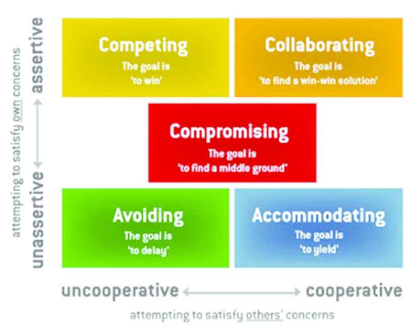
Solving conflict with Nash equilibrium.
Nash equilibrium is a widely utilized model to comprehend the contention between numerous players. For example, the two detainees question, if two detainees are scrutinized a similar interest that on the off chance that he concedes the other individual has made the wrongdoing, he can has ten years rebuff by detainment diminished or else both will be placed in prison for a long time. On the off chance that every one of the two blames the other, that implies a conundrum, both will be placed in prison for a long time. On the off chance that one denounces, the other stay silent, the tranquil individual will get longer discipline.
The conditions of the problem are shown in Table 3.
| AB | Defect | Cooperate |
|---|---|---|
| Defect | 2.2 | 0.3 |
| Cooperate | 3.0 | 1.1 |
The problem circumstances.
By far the best strategy for the prisoners is cooperating to get a short jail term for them both. By contrast, receiving a long jail term is a bad strategy. As it has been pointed out, the problem draws a conflict for each individual in which they do not want to cooperate. It is a choice between competition and cooperation. The agreement to cooperate can guarantees that both win. By contrast, in a noncooperative situation, even a more attractive strategy can lead to worse results.
4.2. A Novel PSO Algorithm Applied for Multi-Round Procurement Problem
PSO [20,55–57] is an advanced computational technique which has been used previously, similar to GA [18], differential evolution (DE) [19], and ant colony optimization (ACO) [25,58,59]. The authors which proposed the algorithm were inspired by the idea of swarm intelligence, as typically seen in animal groups, such as birds, fish, and insects. PSO was first proposed by Russell Eberhart and James Kenedy in 1995 with the main idea of using individual self-experience combined with the social experiences of the entire population. However, the PSO algorithm is not the same as the GA algorithm, as it searches for optima by evaluating individual fitness values based on co-operation and competition among individuals. The PSO algorithm is the consequence of considering a herd of feathered creatures finding sustenance in a specific area. It is a metaheuristic algorithm based on the concept of swarm intelligence, which is useful in solving complex optimization problems [20].
In summary, the PSO algorithm implements a heuristic search through a technique that depends on joining every particle’s conduct and the entire swarm’s conduct by modeling an organic population. The distinction between the PSO and GA algorithms is extremely delicate. Both of them utilize the idea of ensuring the balance of the diversity of the population and similarly rely upon the information shared between their population to elevate their inquiry forms by joining probabilistic and deterministic standards. Therefore, they bring about similar arrangement quality. The idea which distinguishes PSO is its use of neighborhoods. Dissimilar to other heuristic search techniques, in PSO, every particle’s neighborhood is kept invariant. Experimental studies have shown that the PSO algorithm exhibits better robustness and converges much closer to the global optimum than the GA algorithm [20,27,28].
The swarm is comprehended as an accumulation containing various particles which impact the calculation productivity. Be that as it may, particles can be picked haphazardly by and large. A population of particles is initialized with arbitrary speeds and positions, and the wellness capacity is assessed by utilizing a particle’s location and direction. The process initiates the population of particles (N) with some random values for position X and velocity V.
Position:
Velocity:
Each particle maintains knowledge of its best previous evaluated position, represented as
4.2.1. Initialize particles
The representation step plays an important role in the successful design of PSO-MRP algorithm, which aims at finding an appropriate mapping between problem solution and PSO-MRP particle. Assuming that N particles form a population, each particle in the initial solution for the problem was generated randomly. A chromosome is the set of strategies selected for each generation. The best global chromosome found can be considered as the Nash equilibrium point, and the chromosomes in each generation are candidates for the Nash equilibrium point.
The chromosome should bring useful information to represent the solution for the multi-round procurement problem. We propose the format of the Nash equilibrium

Nash equilibrium’s format.
A generation includes the number of rounds in procurement, where each round contains bidding and player information. In the first generation, the estimation of the fitness value of every player is random.
4.2.2. Parameters selection
In each new generation, the algorithm performs the following steps:
Step 1: Call the fitness function and provide fitness values to adjust the priority of particles.
Step 2: Adjust the optimal solution (i.e., global optimum).
Step 3: Update the speed vectors.
Parameters selection of PSO-MRP will play an important role in performance and efficiency of the algorithm. Based on the analysis of the problem, this paper propose an PSO-MRP with the following parameters as shown in Table 4.
| Parameters Name | Variable | Value |
|---|---|---|
| Number of particles | 100 | |
| Number of iterations | 1000 | |
| Inertia weight | 0.4 and 0.9 | |
| Cognitive coefficient | 0.5 | |
| Social component | 0.5 | |
| Stopping criteria | StopCondition | 1000 |
Selected control parameters in PSO-MRP algorithm for multi-round procurement problem.
4.2.3. Fitness function
Multi-stage procurement has a lot of cases and possibilities which can happen, considering the extra conditions given by bidders and investors in order to gain satisfactory benefits. Hence, the constraints considered were as follows:
The whole project is divided into many stages, where the total time of each round equals the project length and each round lasts at least 1 month;
Bidders joining must provide sufficient materials and participate until the end of the project. Moreover, they can join at any stage they want, within their capability.
The constants used are the values that maintain the balance of adaptive function factors. These constants have the role of adjusting the fitness function, in order to direct all of the particles to convergence while satisfying the criteria to get the best result. This function is used to ensure the benefit of both sides in obtaining the maximum profits. Therefore, a solution to optimize the objective function is required.
Particles are evaluated through a fitness function, the fitness value represents the quality of the solution that the particle expresses and also shows its influence in the population. In this problem, we must bring the Fitness function to a minimum, the fitness value is calculated by
4.2.4. Personal best, global best, and particle update
In each generation, particles are updated by comparing their fitness value to that of their best position pBest in all previous iterations. The pBest value is replaced by a new one, if the current fitness value is better. In the next step, the fitness value of each particle is compared with the global best of the population (gBest), where gBest is replaced if a better fitness value is obtained (see Figure 3).
Outstanding particles.
The model to change nodes is if the gBest member has a lower cost, higher quality, and higher association with the venture proprietor than that of particle i. These criteria help to pick the best possible closeout member with the best cost while ensuring the quality of the items delivered. These models are evaluated as a point. If the criteria are met, the point is raised up; otherwise, they are dropped down by one unit. In the event that the fact is sure, the node will be replaced.
When the
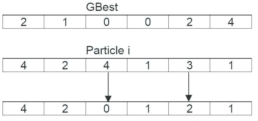
Example of update process.
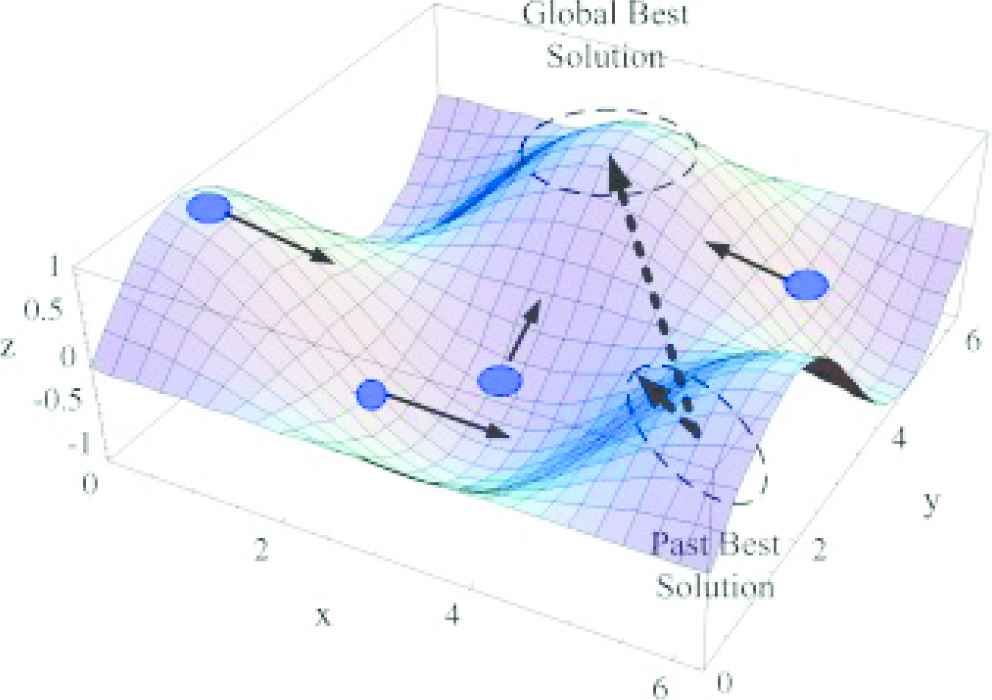
The velocities of particles are updated regularly based on its best experience pBest and the leader gBest. The below equation indicates how
The update of the velocity has been considered an important step since the first generation of development of the PSO-MRP algorithm. Velocity regulation is carried out according to the number of particles that exceed the feasible area during the optimization process. The velocity vector for a particle i is updated according to three other vectors: (i) the personal best position of the
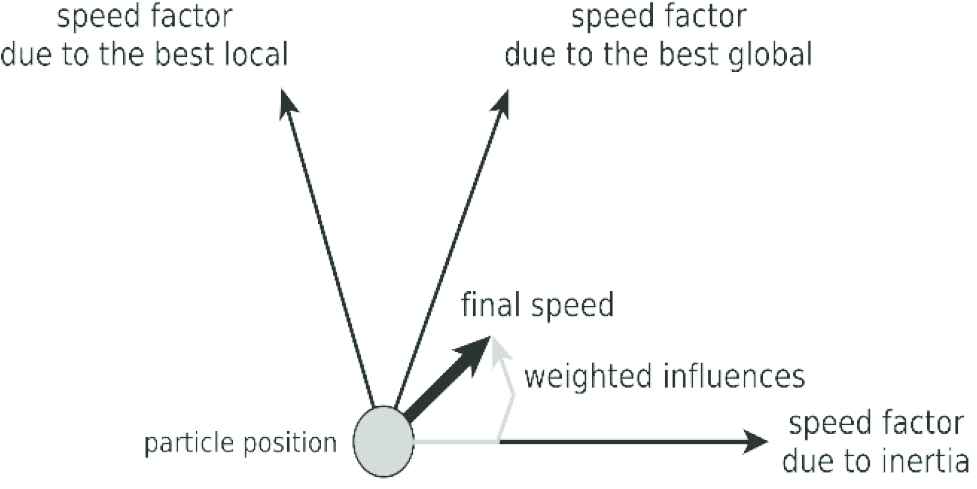
Velocity update process.
The new position is updated by
4.2.5. Stop conditions
For efficient implementation of the PSO-MRP algorithm, we have to determine when to stop iterating. The stop condition of the algorithm can be classified into two techniques:
Firstly, in real-world problems in which a desirable solution range may be available, the stop condition of the algorithm is based on the closeness of the potential solution to this range;
Secondly, the iteration can be stopped when a specific number of generations has been reached.
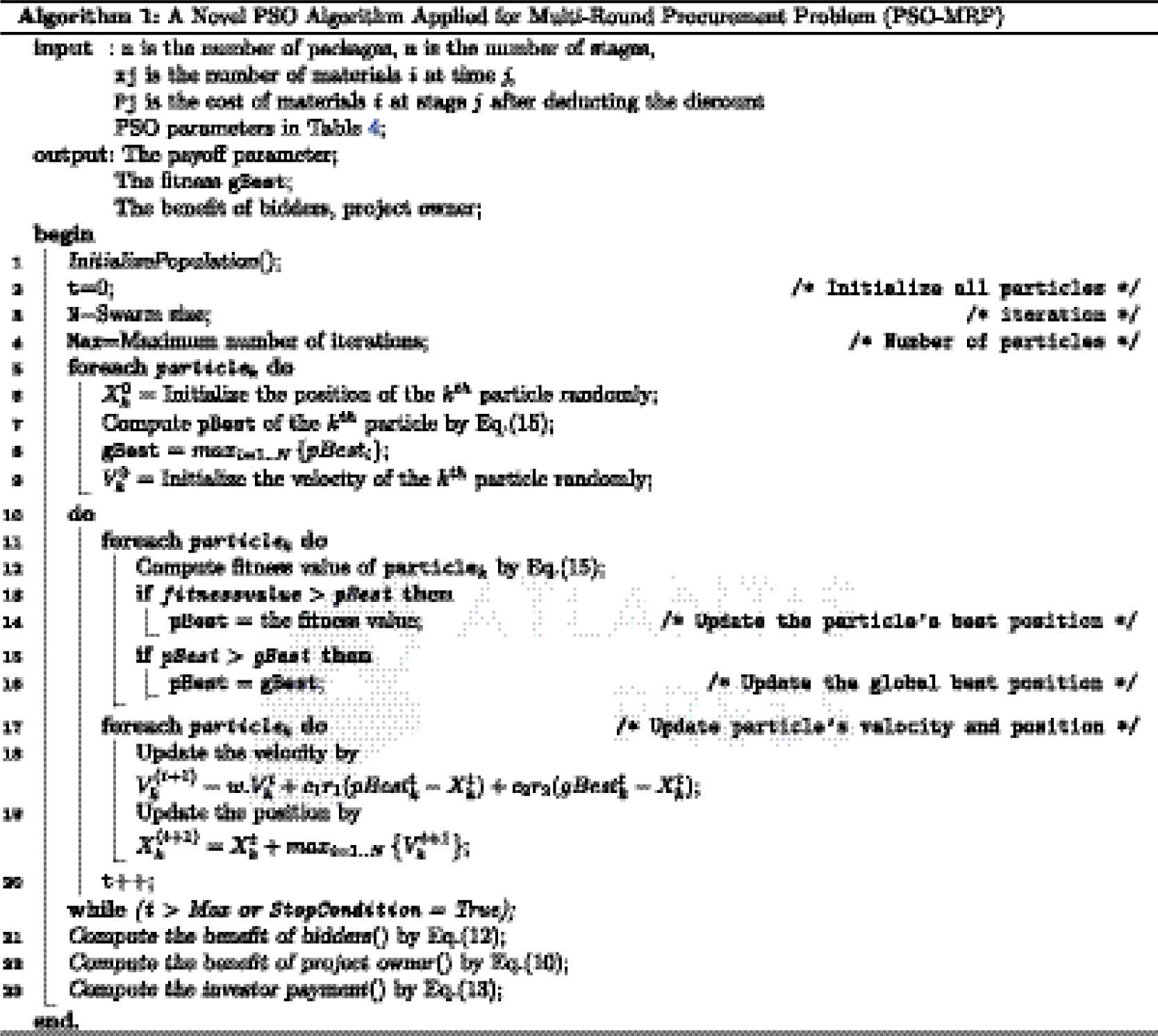
4.2.6. Implementation of PSO-MRP algorithm for multi-round procurement problem
The PSO-MRP algorithm is described in Algorithm 1. Details of the implementation of the PSO-MRP algorithm for multi-round procurement can be found in the supplementary material files.
5. EXPERIMENTS AND RESULTS
5.1. Data Sets
A decision support system based on PSO-MRP was developed to define the Nash equilibrium point for multi-round procurement. The system was written in Java and MySQL. In a real-world project, as most of the procurement data used are kept secret, a large-scale data set for an evolutionary algorithm such as PSO-MRP provides a big obstacle. We found three sample data sets for multi-round procurement in big Vietnamese government-funded projects. The experimental results can prove that a Game-theoretic model and PSO-MRP are suitable in solving a critical and real-world problem in this research. Table 5 shows a summary of the data sets used.
| Data set | Equipment Category | Budget | Number of Bidder |
|---|---|---|---|
| 1 | 46 items | 39.8 billion | 6 |
| 2 | 100 items | 168 billion | 15 |
| 3 | 43 items | 27.6544 million | 5 |
| 4 | 4787 items, 1248 rounds, 2584 proposal | 148,468 billion | 45 |
Summary of data sets.
5.1.1. Data set structure
Data were organized in a .json file with the following structure:
1 {
2 “project_id": “",
3 “inflation_rate": “",
4 “start_date": “",
5
6 “packages": [{
7 “package_id": “",
8 “execution_time" : “",
9 “joined_contractors": [x, xx, xxx],
10 “products": [{
11 “product_id": “",
12 “quantity": “"
13 }],
14
15 “estimated_cost": “"
16 }],
17 “product": [{
18 “product_id": “",
19 “description": “",
20 “unit": “"
21 }],
22
23 “contractors": [{
24 “contractor_id": “",
25 “description": “",
26 “capacity": “",
27 “relationship": “",
28 “products": [{
29 “product_id": “",
30 “sell_price": “",
31 “buy_price": “"
32 }],
33 “strategies": [{
34 “strategy_id": “",
35 “products": [{
36 “product_id": “",
37 “discounts": [{
38 “from": “",
39 “to": “",
40 “rate": “"
41 }]
42 }]
43 }]
44 }]
45 }
5.1.2. Data set description
The summary description of data set 1 and 2 are shown in Tables 6 and 7. The detailed information can be found in the supplementary material files.
| Parameter | Description |
|---|---|
| Project title | IT application investment project in party agencies of Nghe An province. |
| Project duration | From 2015–2020 |
| Budget | Project funded with development investment from the provincial budget, investment limit is 39.8 billion |
| Equipment category | 46 items ( |
| Bidding information | 6 bidders |
| (FPT, HongPhuc, TranAnh, Hanoi ComputerJointStock, Setec, and PhucAnh) |
Detailed information of data set 1.
| Parameter | Description |
|---|---|
| Project title | IT application investment project in party agencies of Haiphong city (2018–2020). |
| Project duration | From 2018 to 2020 |
| Budget | Project funded with development investment from the provincial budget, investment limit is 168 billion |
| Equipment category | 100 items ( |
| Bidding information | 15 bidders |
Detailed information of data set 2.
The project of data set 3 had an total estimated cost is 27,654,400 VND. During the project duration (from 1/1/2019 to 21/6/2019), it was divided into six main packages auctioned in different stages. A total of 43 products were assessed in the unit, and five contractors joined the project. The information contains their company names, their qualities, their relationships with the investor, the discount rate and its time-line, the price contractors bought the products for, and the price they sold them for. The summary description of data set 3 is shown in Table 8; for detailed information, see the supplementary material files.
| Parameter | Description |
|---|---|
| Project title | IT application investment project in party agencies of Hanoi city. |
| Project duration | From 1/1/2019 to 21/6/2019 |
| Total estimated cost | 27,654,400 VND |
| Number of products | 43 |
| Number of contractors | 5 |
Detailed information of data set 3.
Data set 4 is a large-scale project which needs a large number of bidders, resources, items, proposals, and budgets. The project title was IT application investment project in party agencies of Haiphong city (2019–2020) with 4787 items in procurement, 45 bidders joining in the auction of 1248 rounds, each round including several items in the auction. In total, the problem contained 2584 proposals for 8715 items in packages. The summary description of data set 4 is shown in Table 9; detailed information can be found in the supplementary material files.
| Parameter | Description |
|---|---|
| Project title | IT application investment project in party agencies of Haiphong city (2019–2020) |
| Project duration | From 1/1/2019 to 31/12/2019 |
| Budget | 148,468 billion VND |
| Equipment category | 4787 items ( |
| Bidding information | 45 bidders ( |
| Number of proposal | 2584 proposals |
| Number of items in packages | 8715 ( |
Detailed information of data set 4.
5.2. Testing Result
5.2.1. Testing environment
Our experiments were conducted on a computer configured as shown in Table 10.
| Parameter | Configuration |
|---|---|
| CPU | Intel Core i5 6200U (Skylake), 2.7GHz |
| RAM | 8 GB |
| Operating System | Windows 10 Pro |
| Programming language | Java 11, json-simple-1.1.1.jar |
Testing environment.
5.2.2. Case study 1
In the first experiment, we installed and compared the performance of six algorithms, GDE3 (The third evolution step of generalized DE) [29], Multi-Objective Evolutionary Algorithm(
After testing the program 10 times, the populations were randomly initialized, including 100 individuals; the maximum number of individuals created for each runtime was 10,000. The comparison of the payoff parameter and the runtime on data set 1 is given in Table 11. We compare the performance of our algorithm and other algorithms, in terms of best, worst, and average, in Figure 6.
| NSGA-III [35] |
GDE3 [29] |
PESA2 [33] |
PSO-MRP |
|||||||||
|---|---|---|---|---|---|---|---|---|---|---|---|---|
| Ord | Payoff | Time | Payoff | Time | Payoff | Time | Payoff | Time | Payoff | Time | Payoff | Time |
| 1 | 0.2961 | 4.197 | 0.2755 | 6.602 | 0.2805 | 5.981 | 0.2741 | 3.630 | 0.2744 | 8.954 | 0.2805 | 4.300 |
| 2 | 0.3322 | 4.178 | 0.2714 | 6.633 | 0.2799 | 5.992 | 0.2743 | 3.051 | 0.2765 | 8.921 | 0.2811 | 4.369 |
| 3 | 0.2911 | 4.209 | 0.2711 | 6.590 | 0.2799 | 5.974 | 0.2747 | 3.555 | 0.2801 | 8.933 | 0.2816 | 4.321 |
| 4 | 0.2966 | 4.166 | 0.2706 | 6.602 | 0.2811 | 6.000 | 0.2751 | 3.525 | 0.2809 | 9.102 | 0.2796 | 4.256 |
| 5 | 0.2979 | 4.178 | 0.2754 | 6.613 | 0.2821 | 5.981 | 0.2714 | 3.617 | 0.2712 | 8.990 | 0.2801 | 4.273 |
| 6 | 0.3025 | 4.184 | 0.2755 | 6.595 | 0.2797 | 6.112 | 0.2777 | 3.504 | 0.2708 | 9.051 | 0.2823 | 4.291 |
| 7 | 0.3105 | 4.189 | 0.2723 | 6.621 | 0.2797 | 5.969 | 0.2750 | 3.550 | 0.2714 | 8.915 | 0.2841 | 4.315 |
| 8 | 0.2923 | 4.171 | 0.2746 | 6.608 | 0.2810 | 5.980 | 0.2707 | 3.544 | 0.2721 | 8.956 | 0.2800 | 4.324 |
| 9 | 0.2940 | 4.190 | 0.2704 | 6.615 | 0.2807 | 5.987 | 0.2721 | 3.601 | 0.2725 | 8.937 | 0.2799 | 4.210 |
| 10 | 0.3025 | 4.178 | 0.2705 | 6.601 | 0.2805 | 5.994 | 0.2733 | 3.539 | 0.2708 | 8.929 | 0.2796 | 4.356 |
Note: NSGA, non-dominated sorting genetic algorithm; MOEA, multi-objective evolutionary algorithm; GDE3 3rd evolution step of generalized DE; PESA2, strength pareto evolutionary algorithm 2; PSO, particle swarm optimization; MRP, multi-round procurement. Reply
Comparison of the payoff parameter and runtime (seconds) on data set 1.
Figure 6 shows the difference in convergence and stability of the considered algorithms. The proposed PSO-MRP algorithm met both criteria, showing good convergence in the fitness function and fast execution.
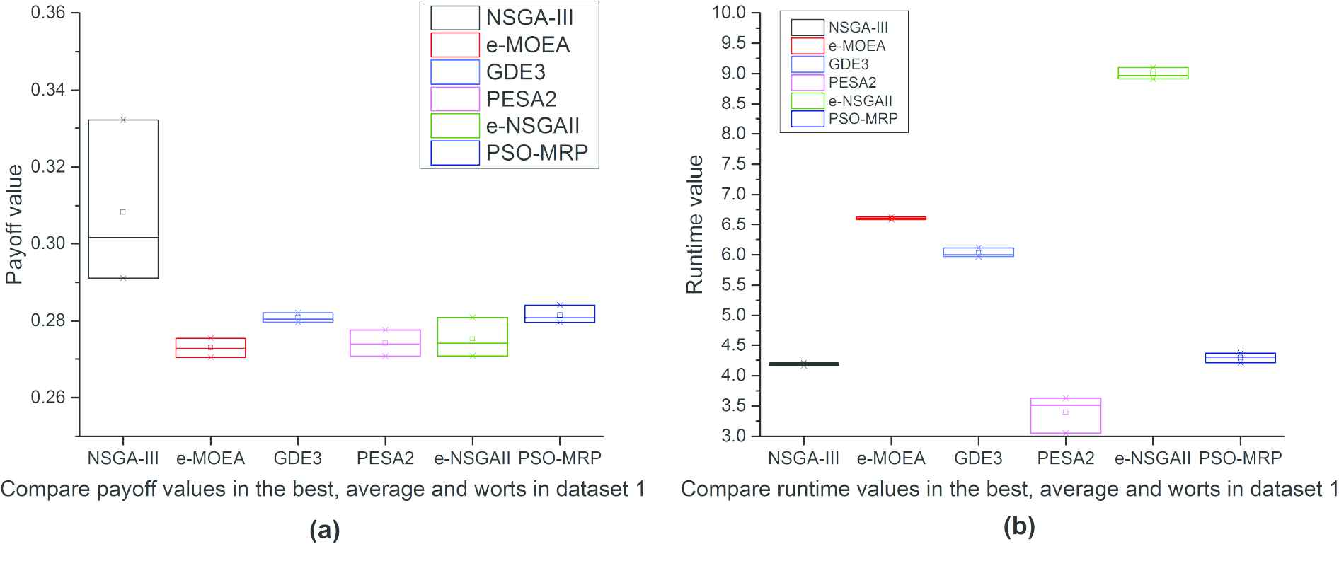
Comparison of payoff and runtime (second) in the best, average, and worst results in data set 1.
5.2.3. Case study 2
In the second experiment, we performed the same experiment as in case study 1 on data set 2. The comparison of the payoff parameter and the runtime on data set 2 is given in Table 12. We also compare the performance of our algorithm and other algorithms, in terms of the best, worst, and average, in Figure 7.
| NSGA-III [35] |
GDE3 [29] |
PESA2 [33] |
PSO-MRP |
|||||||||
|---|---|---|---|---|---|---|---|---|---|---|---|---|
| Ord | Payoff | Time | Payoff | Time | Payoff | Time | Payoff | Time | Payoff | Time | Payoff | Time |
| 1 | 0.2674 | 5.6390 | 0.2590 | 7.6990 | 0.2555 | 7.5150 | 0.2671 | 5.6690 | 0.2555 | 12.4990 | 0.2569 | 5.4960 |
| 2 | 0.2654 | 5.6360 | 0.2596 | 7.6960 | 0.2545 | 7.5170 | 0.2702 | 5.6470 | 0.2569 | 12.5010 | 0.2555 | 5.4750 |
| 3 | 0.2666 | 5.6330 | 0.2610 | 7.7210 | 0.2569 | 7.4860 | 0.2666 | 5.6210 | 0.2518 | 12.4200 | 0.2547 | 5.5020 |
| 4 | 0.2668 | 5.6230 | 0.2591 | 7.7100 | 0.2518 | 7.4970 | 0.2697 | 5.5870 | 0.2525 | 12.4250 | 0.2603 | 5.5140 |
| 5 | 0.2697 | 5.6990 | 0.2610 | 7.6550 | 0.2581 | 7.5250 | 0.2653 | 5.5920 | 0.2522 | 12.3870 | 0.2522 | 5.4770 |
| 6 | 0.2701 | 5.5870 | 0.2586 | 7.6470 | 0.2525 | 7.5290 | 0.2666 | 5.6210 | 0.2557 | 12.4650 | 0.2518 | 5.4210 |
| 7 | 0.2670 | 5.6210 | 0.2589 | 7.6960 | 0.2533 | 7.5330 | 0.2701 | 5.5880 | 0.2525 | 12.4690 | 0.2555 | 5.4330 |
| 8 | 0.2655 | 5.6520 | 0.2587 | 7.7100 | 0.2529 | 7.5290 | 0.2655 | 5.6490 | 0.2551 | 12.4700 | 0.2569 | 5.4350 |
| 9 | 0.2654 | 5.6270 | 0.2590 | 7.6990 | 0.2519 | 7.6000 | 0.2654 | 5.6760 | 0.2543 | 12.4340 | 0.2566 | 5.4150 |
| 10 | 0.2680 | 5.6190 | 0.2599 | 7.6870 | 0.2520 | 7.5550 | 0.2680 | 5.6960 | 0.2569 | 12.4530 | 0.2589 | 5.4500 |
Note: NSGA, non-dominated sorting genetic algorithm; MOEA, multi-objective evolutionary algorithm; GDE3 3rd evolution step of generalized DE; PESA2, strength pareto evolutionary algorithm 2; PSO, particle swarm optimization; MRP, multi-round procurement.
Comparision of payoff parameter and runtime (seconds) on data set 2.
Figure 7 shows the differences in convergence and stability of the considered algorithms. The proposed algorithm had the best runtime.
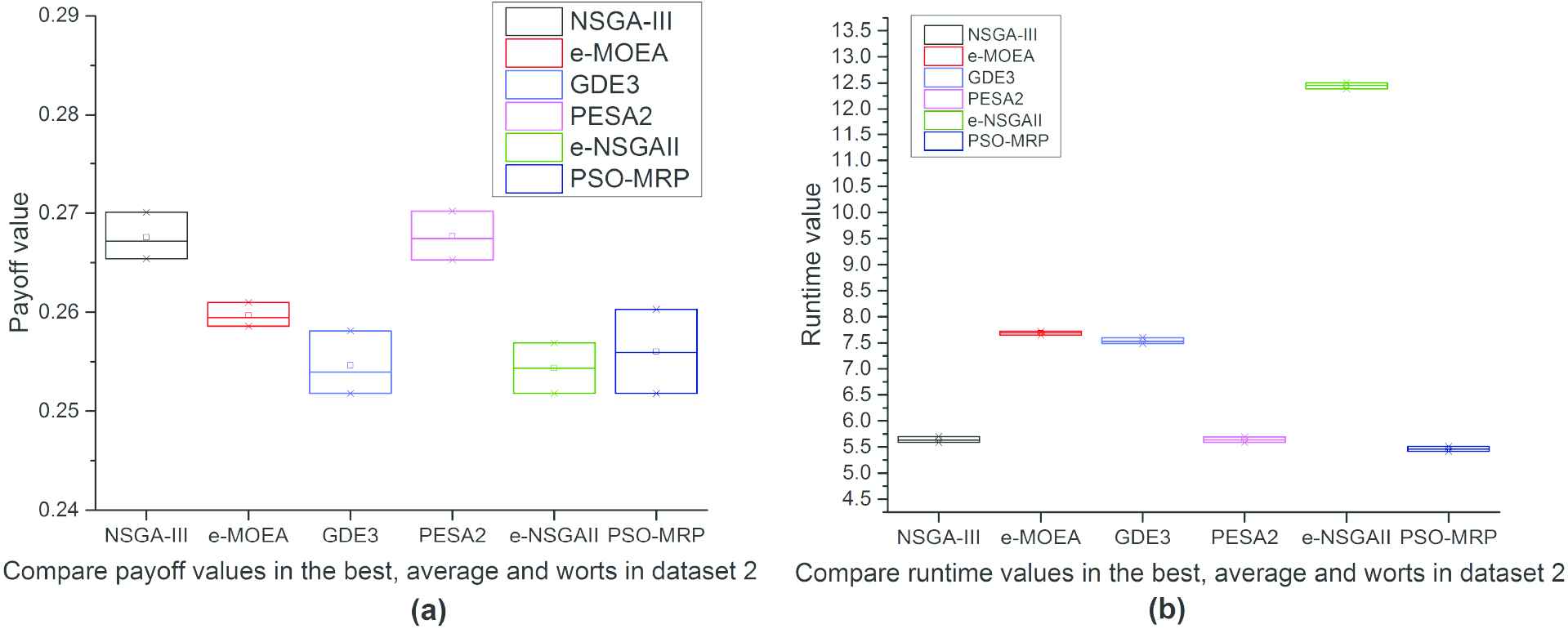
The comparison of payoff and runtime (second) in the best, average, and worst results in data set 2.
5.2.4. Case study 3
After testing the program 10 times, the result of the solution is listed below:
1 Nash Equilibrium found as follows:
2 Number of particles: 10
3 The Nash solution:
4 Chromosome:
5 [4 0 4 2 1 0 ]
6
7 Fitness: 30642322
8 The benefit of bidders: 23624700
9 Bidder0: 128295300
10 Bidder1: 65719300
11 Bidder2: 3999400
12 Bidder3: 0
13 Bidder4: 38233000
14
15 The benefit of project owner: 14472956
16 Investor payment: 13181444
17 Estimated price: 27654400
18
19 Successfully obtained after 0 hours 6 minutes 5 seconds
The comparison of fitness and runtime (minutes) of our algorithm on data set 3 is shown in Table 13. Our proposed algorithm demonstrated stability and convergence of estimated cost and payment values in different experiments.
| Investor (thousand VND) |
Bidder (thousand VND) |
|||||||||
|---|---|---|---|---|---|---|---|---|---|---|
| Ord | Time | Fitness | Estimated cost | Payment | Benefit | 0 | 1 | 2 | 3 | 4 |
| 1 | 6:05 | 33476600 | 27654400 | 13181444 | 14472956 | 2211446 | 143314 | 79090 | 0 | 157556 |
| 2 | 6:08 | 29213000 | 27654400 | 13181444 | 14472956 | 1458516 | 143314 | 183402 | 0 | 224774 |
| 3 | 5:55 | 32380516 | 27654400 | 13181444 | 14472956 | 2211446 | 283406 | 39994 | 0 | 157556 |
| 4 | 5:51 | 29300604 | 27654400 | 13181444 | 14472956 | 1542919 | 138075 | 183402 | 0 | 157556 |
| 5 | 5:51 | 28376784 | 27654400 | 13181444 | 14472956 | 1204395 | 283406 | 18340 | 0 | 224774 |
| 6 | 6:13 | 31539874 | 27654400 | 13181444 | 14472956 | 940112 | 657193 | 39994 | 0 | 690008 |
| 7 | 6:08 | 27531258 | 27654400 | 13181444 | 14472956 | 940112 | 423862 | 183402 | 0 | 233302 |
| 8 | 6:10 | 29300604 | 27654400 | 13181444 | 14472956 | 1542919 | 138075 | 183402 | 0 | 157556 |
| 9 | 6:28 | 31750880 | 27654400 | 13181444 | 14472956 | 1960984 | 240098 | 79090 | 0 | 224774 |
| 10 | 6:16 | 28376784 | 27654400 | 13181444 | 14472956 | 1204395 | 283406 | 183402 | 0 | 224774 |
Comparision of fitness and runtime (minutes) of our algorithm on data set 3.
Our proposed algorithm shows the stability and convergence of values estimated cost and payment in different experiments. Through experiments shows that the values of estimated cost (27,654,400), investor payment (13,181,444), and benefit of project owner (14,472,956) are not changed. However, the distribution of the bidder values will fluctuate, resulting in a fluctuation in the fitness function (see Table 14)
| Min | Max | Mean | std | |
|---|---|---|---|---|
| Time | 5.51 | 6.28 | 5.945 | 0.29789 |
| Fitness optimal | 27531258 | 33476600 | 30124690.4 | 1999915.156 |
| Bidder 0 | 940112 | 2211446 | 1521724.4 | 474601.161 |
| Bidder 4 | 138075 | 657193 | 273414.9 | 163915.868 |
| Bidder 2 | 18340 | 183402 | 117351.8 | 71889.476 |
| Bidder 4 | 157556 | 690008 | 245263 | 159996.683 |
Analysis and statistical evaluation of time, fitness, bidders’ value of PSO-MRP algorithm in data set 3.
5.2.5. Case study 4
To evaluate the performance and convergence of our algorithm in terms of both the fitness and time functions, we compared the performance between the different meta-heuristic algorithms on a large-scale project in data set 4, which had a large number of bidders, resources, items, proposals, and budgets. The experiment results are listed in Tables 15 and 16, which show that our algorithm had the best performance and quality of Nash equilibrium point when the fitness values were lowest.
| Ord | NSGA-III [35] | GDE3 [29] | PESA2 [33] | PSO-MRP | ||
|---|---|---|---|---|---|---|
| 1 | 1,307,737 | 1,251,764 | 1,028,268 | 1,269,256 | 1,240,694 | 1,055,274 |
| 2 | 1,275,423 | 1,240,213 | 1,087,182 | 1,284,698 | 1,259,906 | 953,342 |
| 3 | 1,280,605 | 1,440,048 | 1,048,430 | 1,289,464 | 1,165,777 | 934,703 |
| 4 | 1,369,824 | 1,113,870 | 1,118,879 | 1,137,605 | 1,142,129 | 998,258 |
| 5 | 1,251,295 | 1,175,737 | 1,171,253 | 1,225,694 | 1,268,246 | 1,064,634 |
| 6 | 1,297,487 | 1,343,591 | 1,186,463 | 1,020,719 | 1,209,126 | 953,237 |
| 7 | 1,390,135 | 1,208,916 | 1,148,664 | 1,294,479 | 1,146,635 | 1,037,284 |
| 8 | 1,362,089 | 1,299,300 | 1,006,452 | 1,046,804 | 1,164,376 | 935,569 |
| 9 | 1,334,285 | 1,123,940 | 1,186,586 | 1,272,498 | 1,145,861 | 998,714 |
| 10 | 1,246,259 | 1,368,942 | 1,164,761 | 1,273,764 | 1,156,935 | 1,090,015 |
NSGA, non-dominated sorting genetic algorithm; MOEA, multi-objective evolutionary algorithm; GDE3 3rd evolution step of generalized DE; PESA2, strength pareto evolutionary algorithm 2; PSO, particle swarm optimization; MRP, multi-round procurement.
Comparison of the fitness values of different algorithms on data set 4.
| Ord | NSGA-III [35] | GDE3 [29] | PESA2 [33] | PSO-MRP | ||
|---|---|---|---|---|---|---|
| 1 | 10m 20s | 15m 43s | 13m24s | 12m 59s | 9m 12s | 7m 07s |
| 2 | 10m 42s | 15m 48s | 13m37s | 14m 36s | 10m 07s | 6m 23s |
| 3 | 11m 6s | 15m 29s | 14m 02s | 15m 13s | 11m 01s | 6m 11s |
| 4 | 9m 53s | 14m 55s | 14m 22s | 14m 23s | 9m 46s | 7m 25s |
| 5 | 9m 48s | 15m 17s | 13m 45s | 12m 15s | 9m 22s | 6m 48s |
| 6 | 11m 27s | 14m48s | 13m 51s | 12m 23s | 10m 56s | 6m 29s |
| 7 | 11m 1s | 14m 35s | 13m 11s | 14m 53s | 8m 54s | 7m 16s |
| 8 | 9m 46s | 16m 01s | 12m 35s | 13m 49s | 9m 36s | 7m 13s |
| 9 | 10m 31s | 15m 24s | 12m 41s | 13m 08s | 9m 57s | 6m 49s |
| 10 | 10m 33s | 15m 47s | 14m 48s | 12m 52s | 10m 24s | 6m 27s |
NSGA, non-dominated sorting genetic algorithm; MOEA, multi-objective evolutionary algorithm; GDE3 3rd evolution step of generalized DE; PESA2, strength pareto evolutionary algorithm 2; PSO, particle swarm optimization; MRP, multi-round procurement.
Comparison of the runtimes of different algorithms on data set 4.
Figure 8 shows the differences in convergence and stability of the considered algorithms. The proposed algorithm had both the best runtime and best fitness.
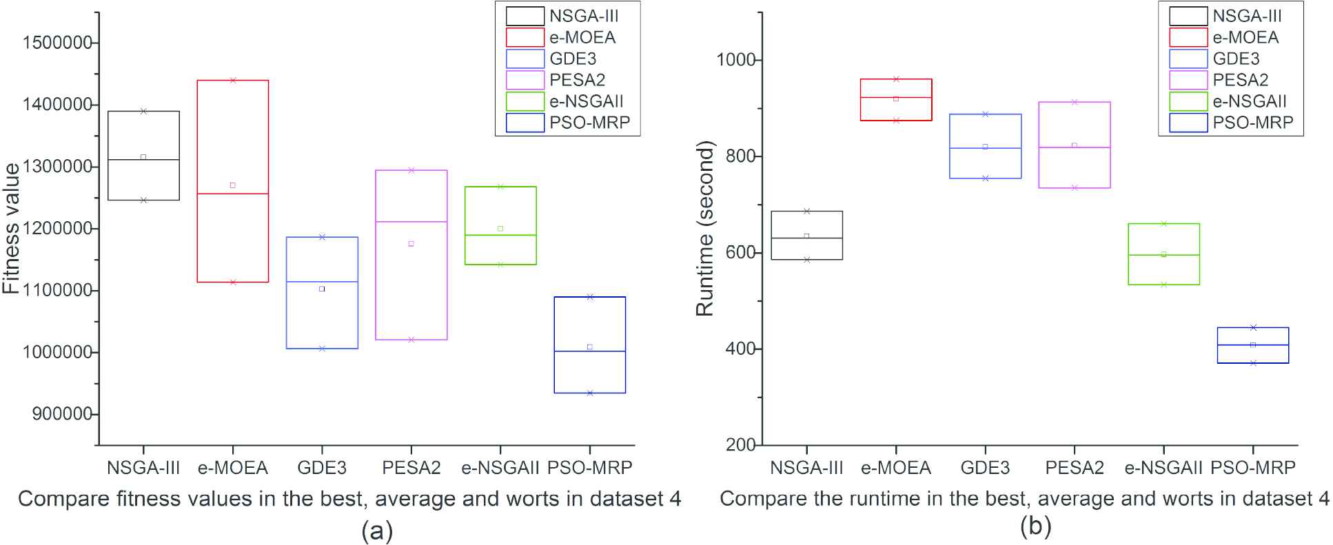
Comparison of fitness and runtime (second) in the best, average, and worst results in data set 4.
5.2.6. Case study 5
In this experiment, the PSO-MRP algorithm was executed 100 times with randomly initialized populations including 100 individuals, where the maximum number of individuals created for each runtime was 10000. We evaluated the stability of the algorithm based on certain parameters, such as the minimum (Min), maximum (Max), mean, variance, and standard deviation (Std) of fitness, as well as time cost, in Tables 17 and 18.
| Payoff value | Time cost (second) | |||||||||
|---|---|---|---|---|---|---|---|---|---|---|
| Dataset | Min | Max | Mean | Variance | Std | Min | Max | Mean | Variance | Std |
| 1 | 0.280 | 0.284 | 0.281 | 2.095E-06 | 0.0014476 | 4.210 | 4.369 | 4.302 | 0.0022183 | 0.0470992 |
| 2 | 0.252 | 0.260 | 0.256 | 7.017E-06 | 0.0026489 | 5.415 | 5.514 | 5.462 | 0.0012731 | 0.0356801 |
Analysis and statistical evaluation of convergence of the proposed PSO-MRP algorithm in data sets 1 and 2.
| Fitness optimal | Time cost (second) | |||||||
|---|---|---|---|---|---|---|---|---|
| Dataset | Min | Max | Mean | Std | Min | Max | Mean | Std |
| 3 | 27,531,258 | 33,476,600 | 28,915,472 | 2315.3072 | 5.51 | 6.28 | 5.945 | 0.297890733 |
| 4 | 934,703 | 1,090,015 | 975,453 | 57,217.74 | 371 | 445 | 409 | 25.667 |
Analysis and statistical evaluation of convergence of proposed PSO-MRP algorithm in data sets 3 and 4.
5.2.7. Discussion
From the experimental results in Tables 4 and 5, the
The order of runtime was similar in the two data sets.
Both the
In both data sets, the NSGA-III algorithm gave the worst results, as it very easily became stuck at local solutions.
The
Both
Similarly, PSO-MRP and GDE3 had in common that the selection was not carried out through a mating process but, instead, was based on an individual transformation (mutation, or change in rules); therefore, the resulting orders had similarities in the two data sets.
From overall observation, the authors drew some conclusions for case study 3:
The result after each run converged and shared a similar solution.
Contractors were likely to have similar interests.
The choosing decision was based on many other criteria, such as the price, the relationship, and the quality of each bidder. However, more trustworthy contractors were more likely to be chosen; especially bidder 3, which did not have any relationship with the investor.
The program took some time and depended on the size of the swarm population and the max running fold.
The proposed PSO-MRP algorithm met both criteria, demonstrating good convergence in the fitness function and fast execution. Our algorithm can, thus, provide the best performance in terms of payoff and time taken with limited iterations, as seen in case studies 4 and 5.
6. CONCLUSION
This paper at hand presents a novel approach on how to combine Game theory and PSO algorithm to support decision-making in the multi-round of an auction. In the first phase, we propose a game model which brings all needed information, criteria, and constraints of the problem. In the second phase, the PSO algorithm is utilized with a suitable set of parameters to figure out the Nash equilibrium point. We proved that conflict, such as the competition and cooperation in multi-round procurement, can be resolved by defining a sustainability strategy that brings all participants of the problem into a win-win solution. Additionally, the model was successfully applied in our experiments, demonstrating the usefulness of the Nash equilibrium point for the multi-round procurement issue.
However, restrictions have not vanished, as procurement is typically a secure project. Therefore, the data gathering process encountered many difficulties and information was ultimately lacking. Moreover, the program requires an optimized solution and may need to be run several times to get the best result. Some unexpected risks and issues during the project were not calculated. Therefore, it is still necessary to do more experiments and research to develop an optimized method.
For future research, the authors wish to improve the optimization of the algorithm, reduce the time cost to run the program, and complete the software development.
CONFLICTS OF INTEREST
The authors have declared no conflicts of interest.
ACKNOWLEDGMENTS
This research is funded by Vietnam National Foundation for Science and Technology Development (NAFOSTED) under grant number 102.03-2019.10.
REFERENCES
Cite this article
TY  - JOUR
AU  - Trinh Ngoc Bao
AU  - Quyet-Thang Huynh
AU  - Xuan-Thang Nguyen
AU  - Gia Nhu Nguyen
AU  - Dac-Nhuong Le
PY  - 2020
DA  - 2020/09/14
TI  - A Novel Particle Swarm Optimization Approach to Support Decision-Making in the Multi-Round of an Auction by Game Theory
JO  - International Journal of Computational Intelligence Systems
SP  - 1447
EP  - 1463
VL  - 13
IS  - 1
SN  - 1875-6883
UR  - https://doi.org/10.2991/ijcis.d.200828.002
DO  - 10.2991/ijcis.d.200828.002
ID  - Bao2020
ER  -