
Cubic Graphs and Their Application to a Traffic Flow Problem
 , M. Mohseni Takallo2, , Y. B. Jun2, 3, R. A. Borzooei2,
 - DOI
- 10.2991/ijcis.d.200730.002How to use a DOI?
- Keywords
- Cubic set; Interval-valued fuzzy set; Cubic graph; (complete, strong) cubic graph; Cubic (bridge, cutvertex); Traffic flows
- Abstract
A graph structure is a useful tool in solving the combinatorial problems in different areas of computer science and computational intelligence systems. In this paper, we introduce the concept of cubic graph, which is different from the notion of cubic graph in S. Rashid, N. Yaqoob, M. Akram, M. Gulistan, Cubic graphs with application, Int. J. Anal. Appl. 16 (2018), 733–750, and investigate some of their interesting properties. Then we define the notions of cubic path, cubic cycle, cubic diameter, strength of cubic graph, complete cubic graph, strong cubic graph and illustrate these notions by several examples. We prove that any cubic bridge is strong and we investigate equivalent condition for cubic cutvertex. Finally, we use the concept of cubic graphs in traffic flows to get the least time to reach the destination.
- Copyright
- © 2020 The Authors. Published by Atlantis Press B.V.
- Open Access
- This is an open access article distributed under the CC BY-NC 4.0 license (http://creativecommons.org/licenses/by-nc/4.0/).
1. INTRODUCTION
Graph theoretical concepts are widely used to study and model various applications in different areas including computer science, computational intelligence, automata theory, operations research, economics, and transportation. However, in many cases, some aspects of a graph-theoretic problem may be vague or uncertain. Fuzzy graphs were introduced by Rosenfeld [1], ten years after Zadeh's landmark paper “Fuzzy Sets” (briefly
Now, in the real life, some phenomena can be modeled with fuzzy graph concepts and some with interval-valued graph concepts. But there are some more complex phenomena that cannot be expressed alone, and can be modeled with a combination of both, that is cubic graphs. For example, traffic flows.
For this reason, Rashid et al. [18] applied cubic sets on graphs and introduced the notion of cubic graphs. But we thinks that this definition is not correct, since in the special case it is not a fuzzy graph.
So, in this article we introduce the correct notion of cubic graph which is different from the cubic graph in [18]. We define the notions of
2. PRELIMINARIES
A fuzzy set is a pair
By an interval number we mean a closed subinterval
For any
An interval-valued fuzzy set (briefly, an IVF set) on nonempty set
The complement
For a family
Let
Definition 2.1.
[23] Let
Let
Definition 2.2.
[36] A fuzzvgraph
The fuzzy set
Definition 2.3.
[36] By an interval-valued fuzzy graph of a graph
3. CUBIC GRAPHS
In graph theory, there are some very basic concepts that whenever we just want to apply a new structure to graphs, these basic concepts must be introduced in that new structure. These basic concepts include vertex, edge, path, cycle, diameter, bridge, complete graph, sub-graph, and so on. Now in this section, all these important concepts for cubic graphs are stated and the related results are obtained.
Rashid et al. [18] applied cubic sets on graphs and introduced the notion of cubic graphs as follows: Let
But this definition is not correct. Since if
Definition 3.1.
Let
Let
It is clear that any cubic graph is fuzzy graph and interval-valued fuzzy graph.
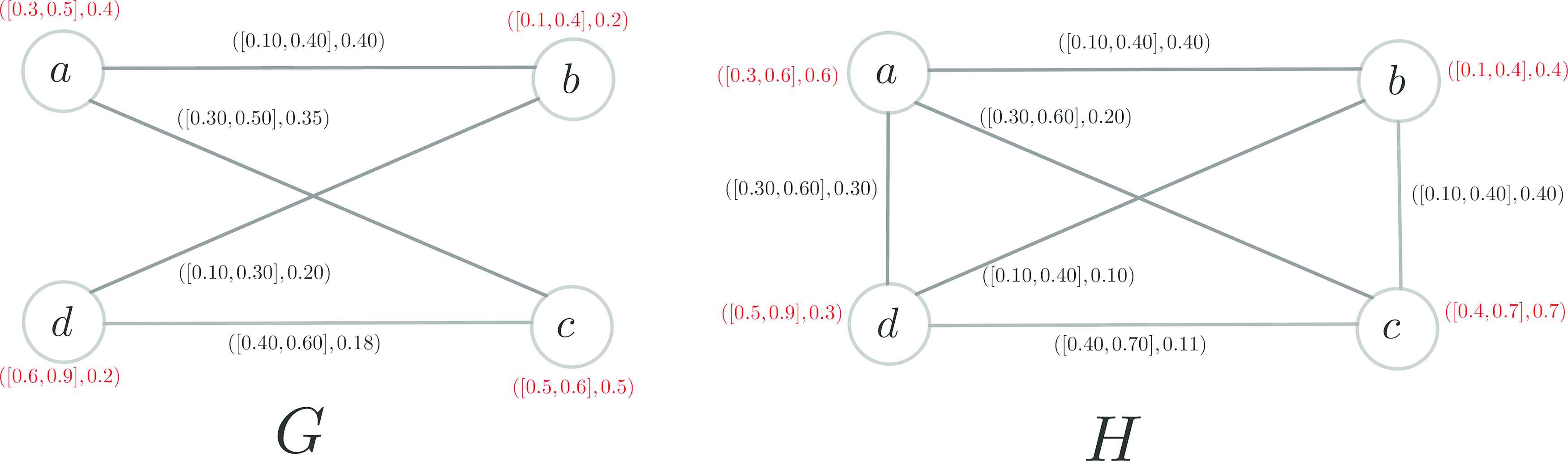
Example 3.2.
Given a set
Tabular representation of “
Tabular representation of “
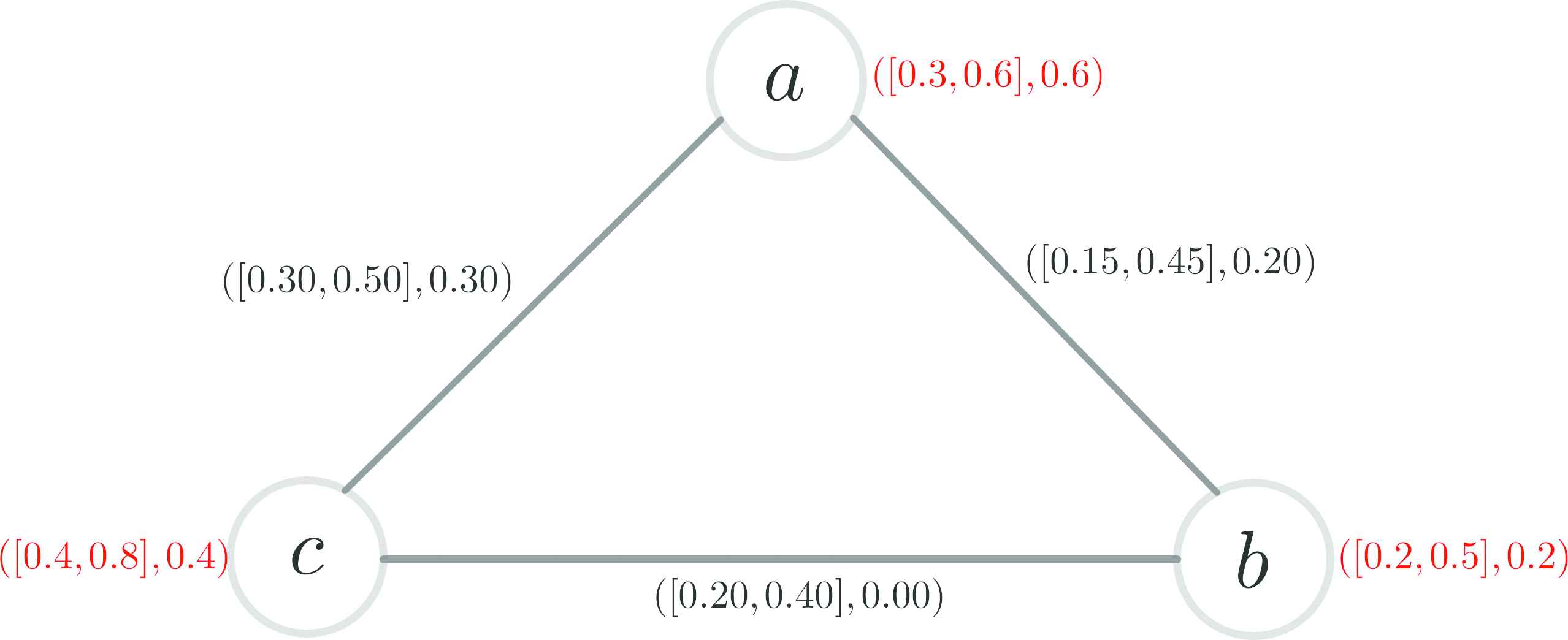
Cubic graph “
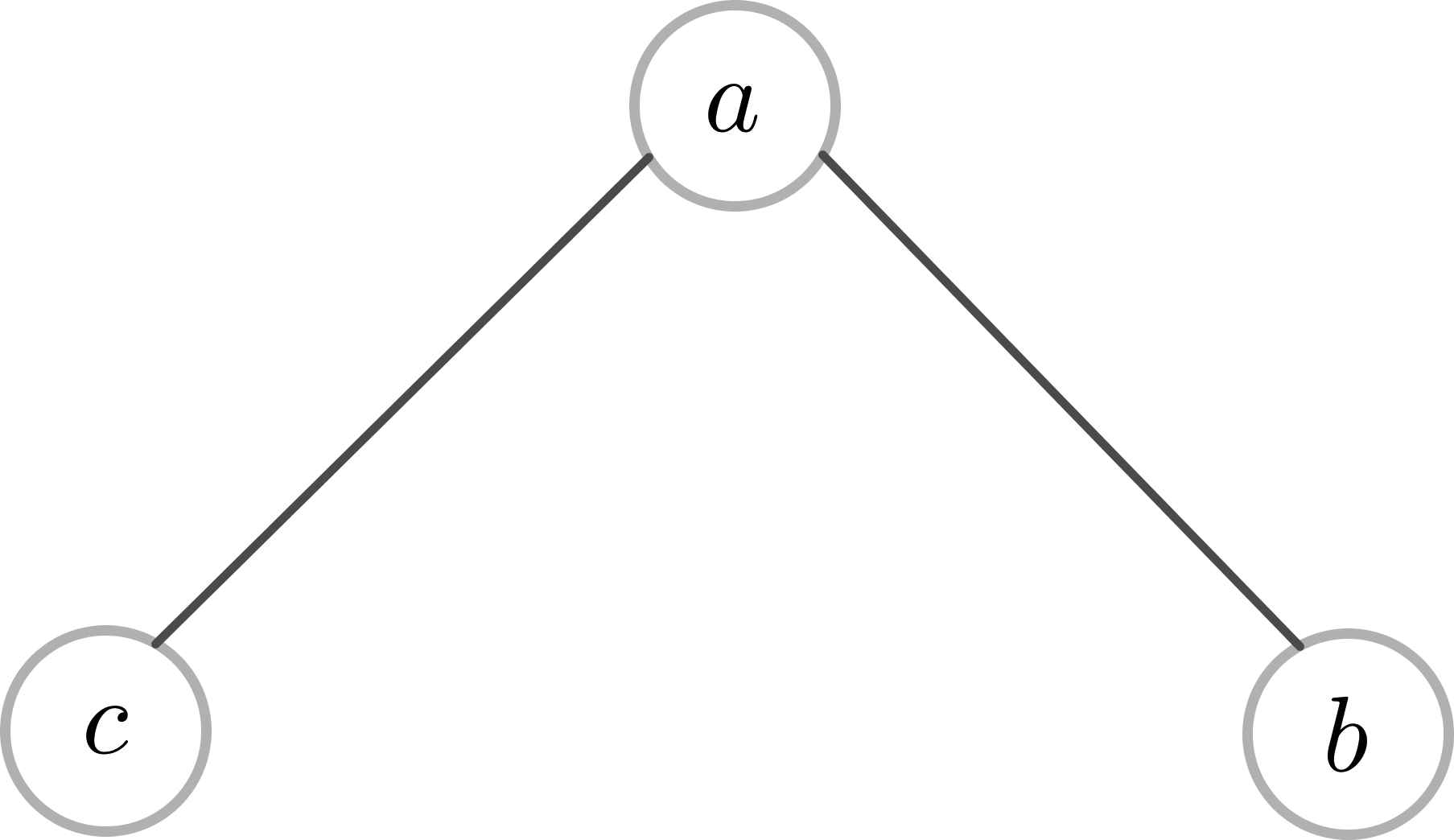
Underlying graph of “G” i.e “
Now, in the following definitions we introduce the concepts of cubic path, cubic cycle, cubic diameter, strength of path, strength of connectedness and complete cubic graph which are necessary for this study and the next results.
Definition 3.3.
Let
An
An
By a cubic path in
By an
By an
By an cubic cycle of length
Definition 3.4.
Let
The
The
The cubic diameter of vertex
Definition 3.5.
Let
The strength of
andGiven an edge
Definition 3.6.
Let
Denote by
Definition 3.7.
A cubic graph
Complete if it is both
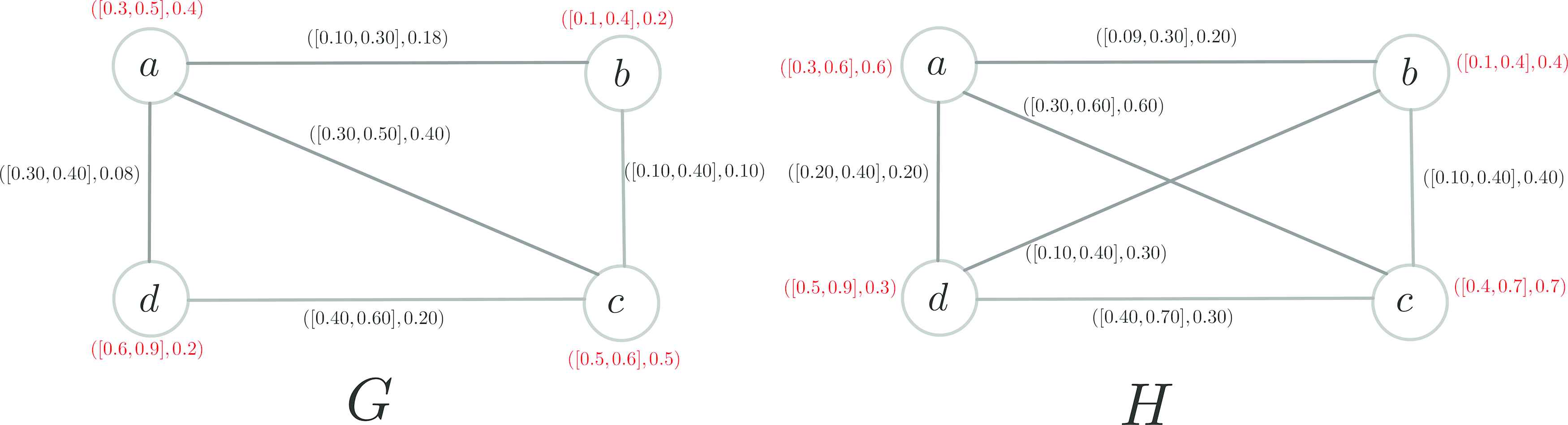
Example 3.8.
Given a set
Tabular representation of “
Tabular representation of “
Then
Complete cubic graph “
Example 3.9.
Let
IVF-Complete cubic graph “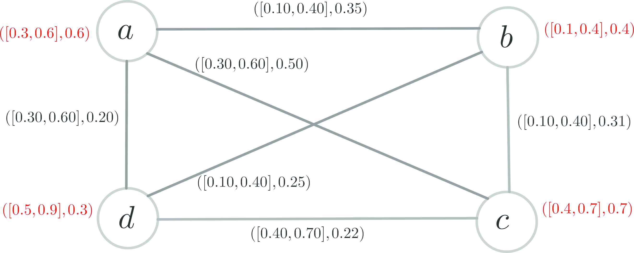
Then
Let F-Complete cubic graph “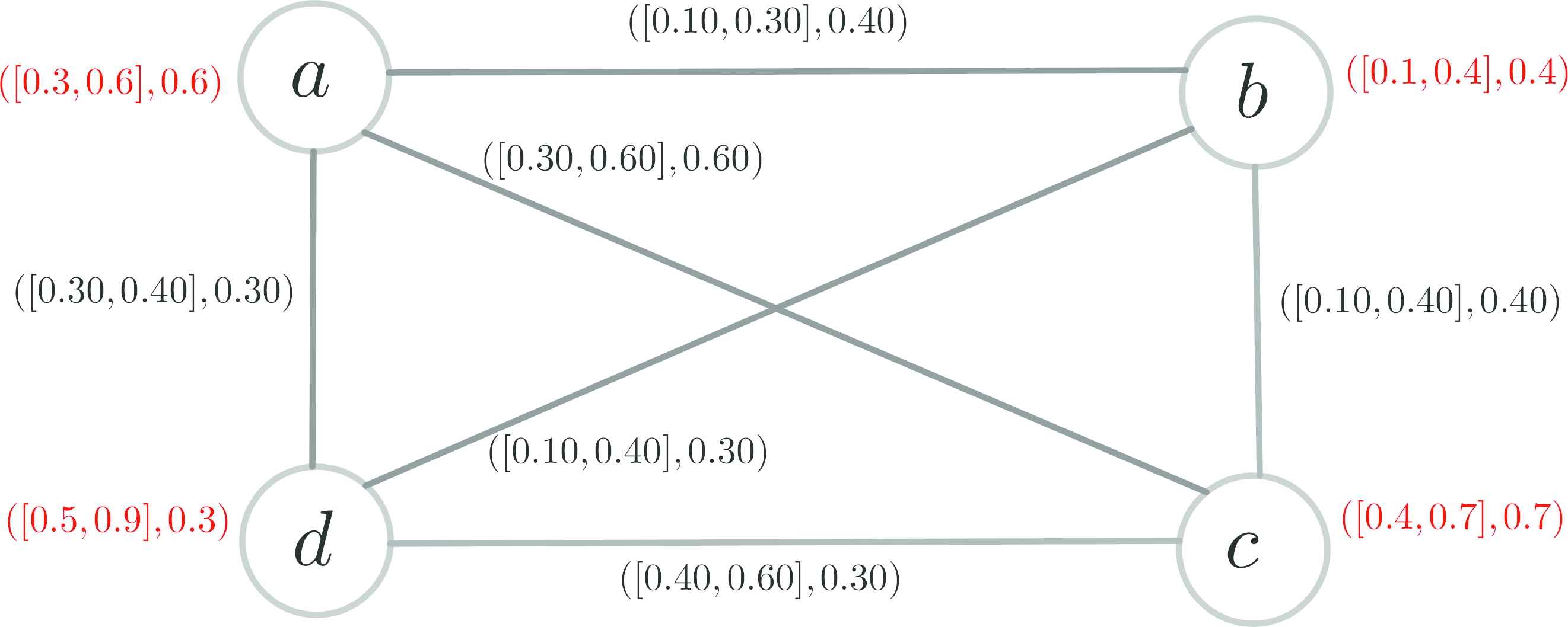
Then
In the following theorem, we determine an upper bound for maximum of strengths in the complete cubic graphs.
Theorem 3.10.
Let
If
If
If
Proof.
(i) and (ii). By using mathematical induction, we know that
(iii) Proof is clear by (i) and (ii).
Definition 3.11.
Let
- where
- where
Strong edge in
Definition 3.12.
Let
Strong if it is both
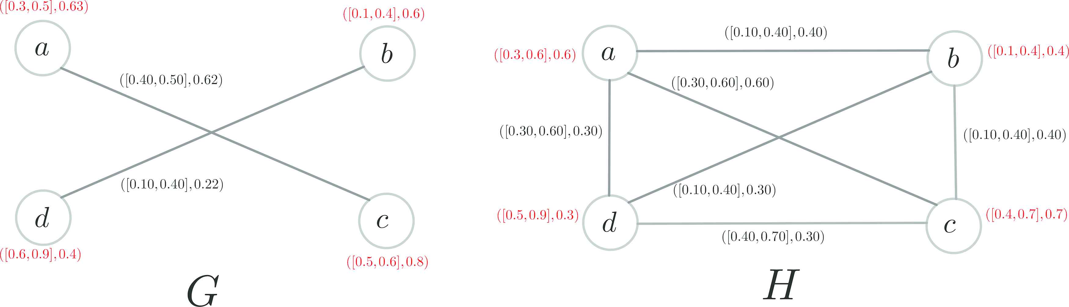
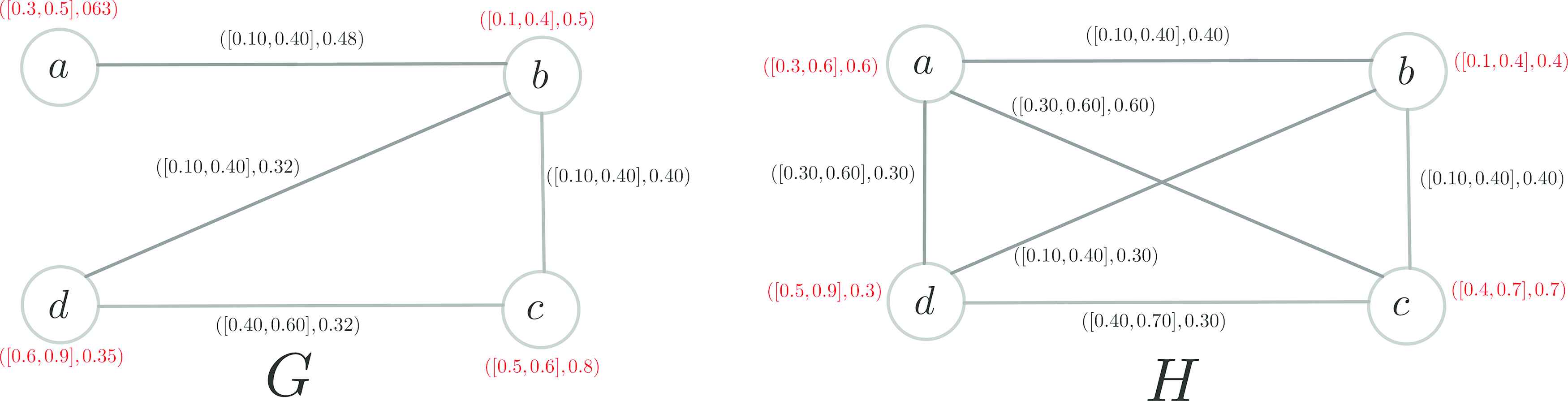
Example 3.13.
Let Cubic graph “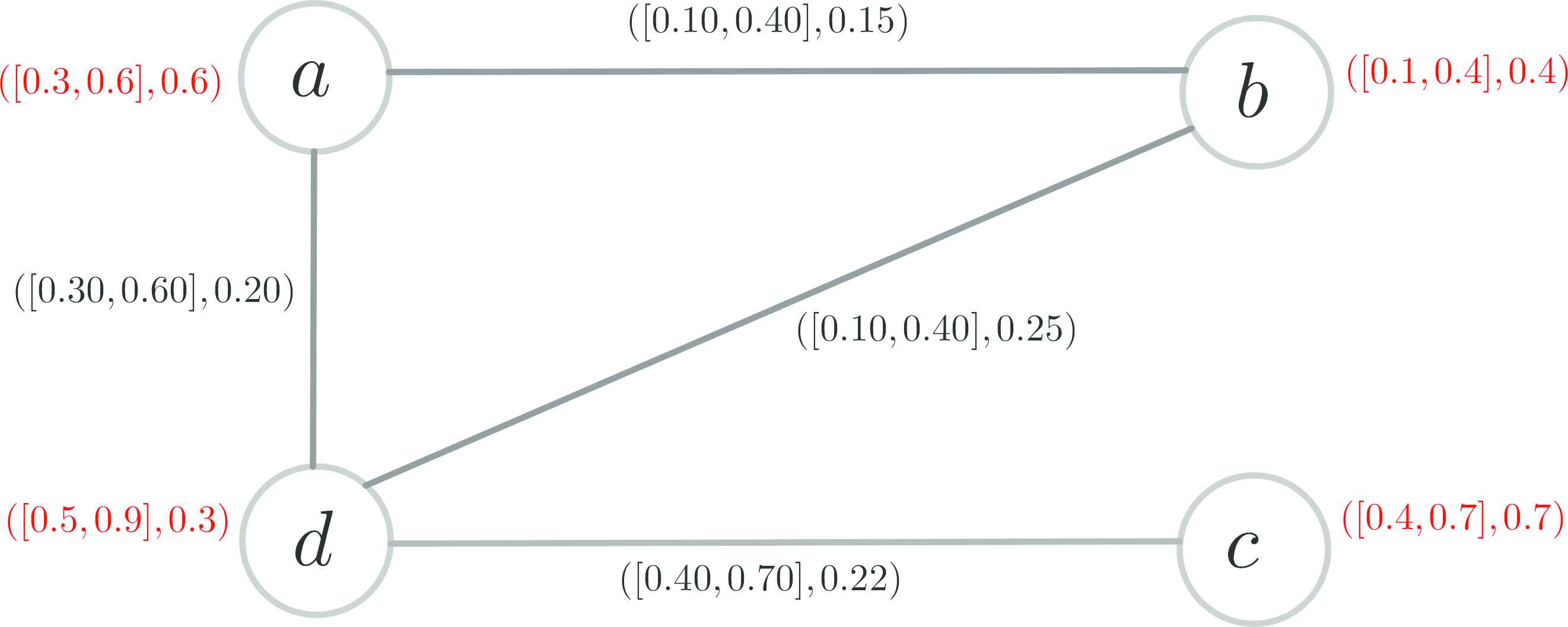
But it is not an
The cubic graph Cubic graph “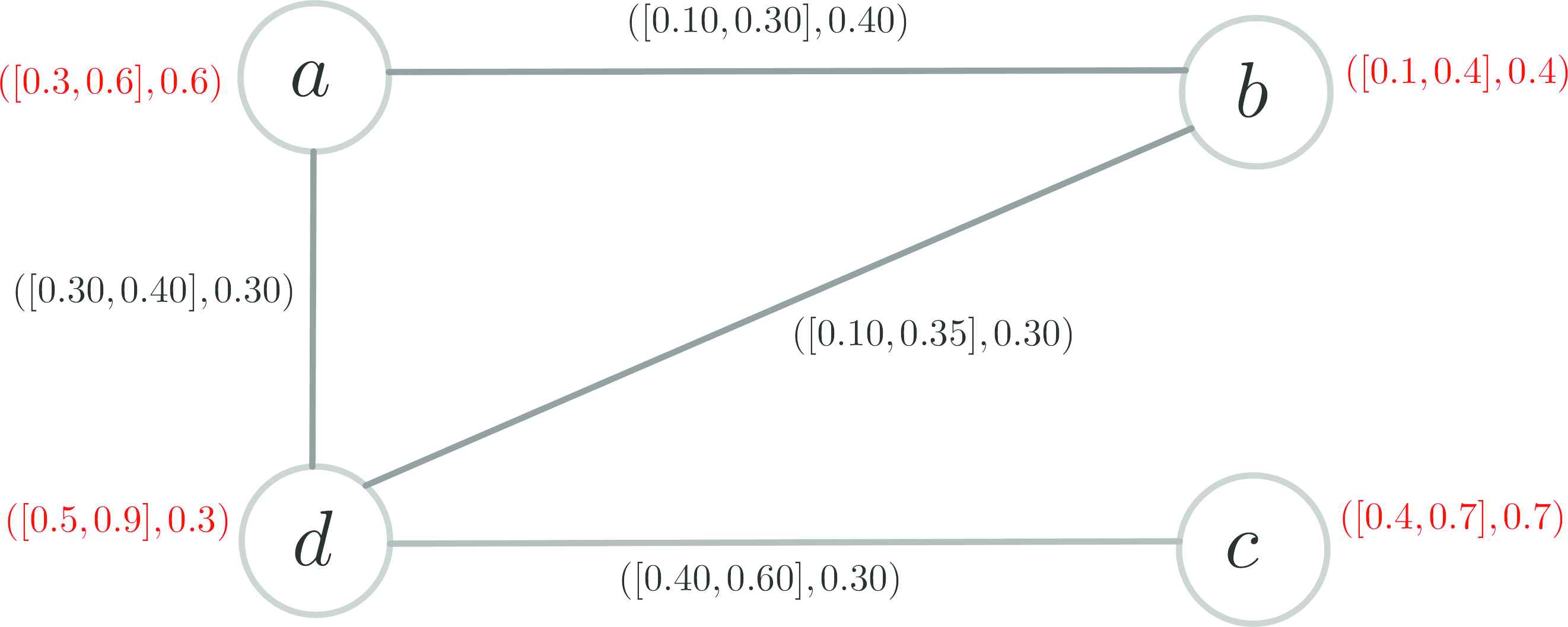
But it is not an
The cubic graph Cubic graph “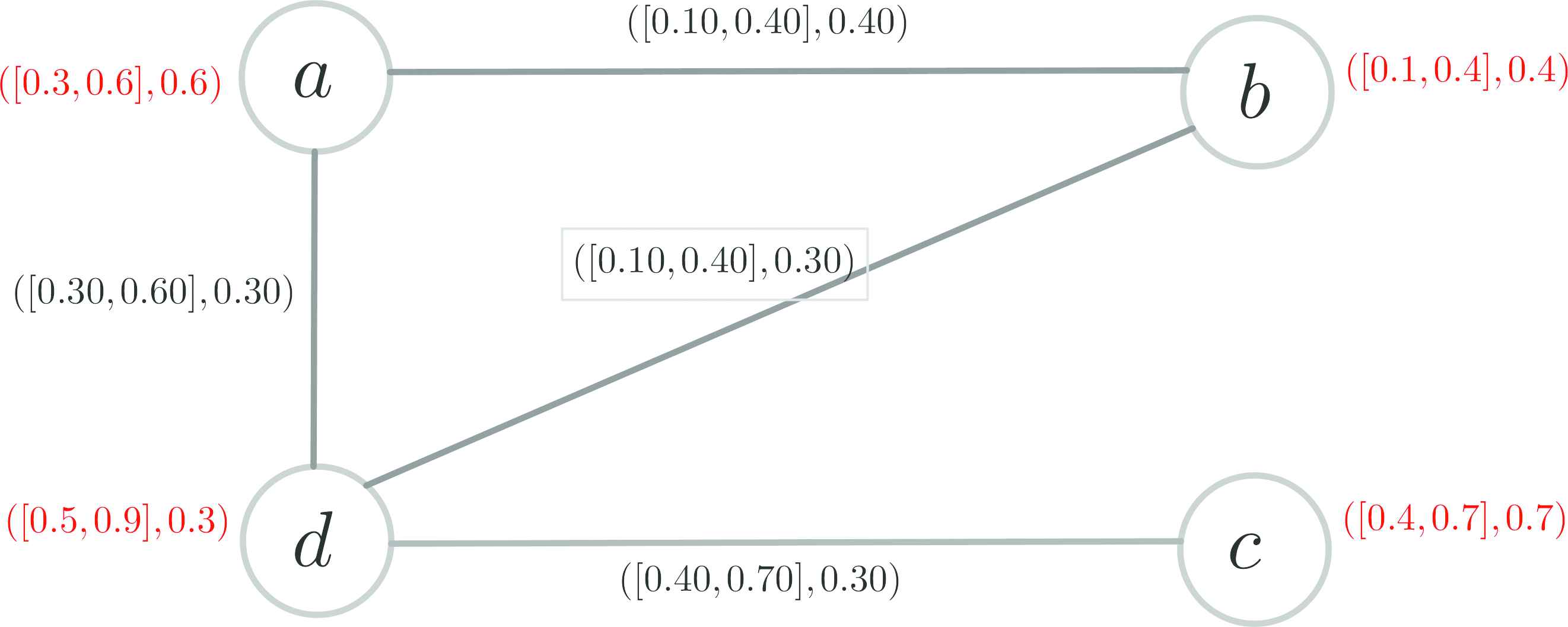
In the following theorems, we investigate some equivalent conditions for (
Theorem 3.14.
Let
Proof.
Assume that
If an
Suppose that
Theorem 3.15.
Let
If
If
If
Proof.
(1) Let
Similarly
(2) Let
Similarly
It follows from 3.7 that
Definition 3.16.
Let
If
If
If
If
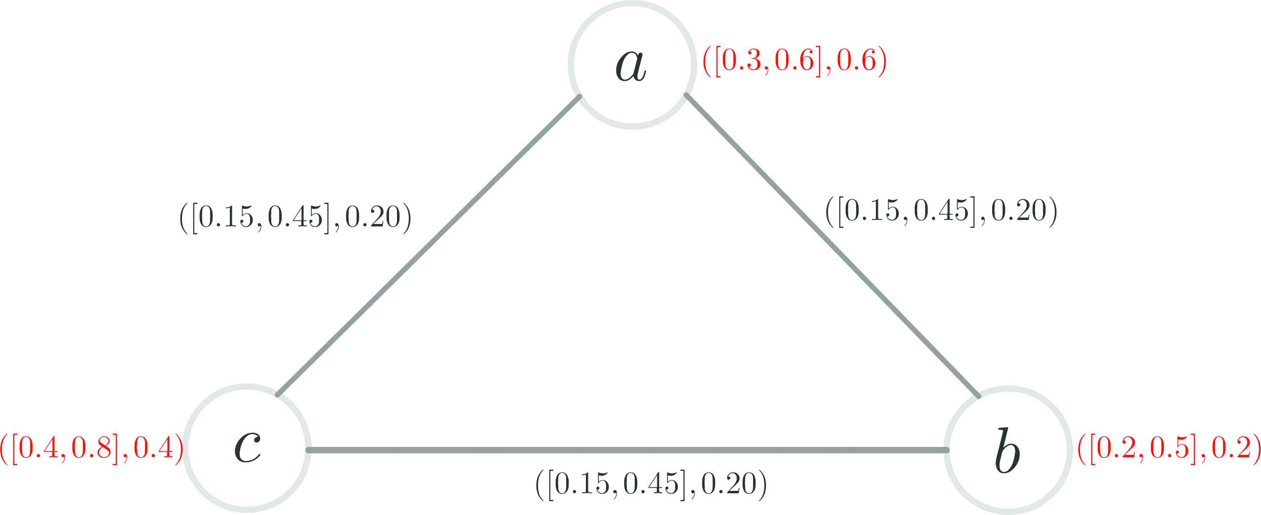
Definition 3.16 is illustrated in the Figures 9–12.
“
“
“
“
Definition 3.17.
Given a cubic graph
Proposition 3.18.
Let
Proof.
The proof is clearly.
Theorem 3.19.
Let
Proof.
If
One of the important results in the fuzzy graph theory, is the relation between bridge, strong arc and cutvertex. Now, in the following theorems we will investigate this relations.
Proposition 3.20.
In a cubic graph
Proof.
Let
Let
The converse of Proposition 3.20 may not be true as seen in Figure 13.
“A strong cycle without cubic bridge.”
Theorem 3.21.
Let
Proof.
By Theorem 3.19 and Proposition 3.20, it is clear.
Definition 3.22.
Given a cubic graph
Proposition 3.23.
Let
Proof.
Straightforward.
Theorem 3.24.
Let
Proof.
Let
Conversely, let
Thus
4. APPLICATION
Traffic flow is the theory, which is developed based on the flow of vehicle on the lane, along with its connections with other vehicles, pedestrians, signals, which is present on the road. Free movement of traffic is affected by many factors like design speed, percentage of heavy vehicles, number of lanes and intersections which are available along the road.
Traffic flow in a road is expressed as number of vehicles using the particular road per unit duration during one hour and is measured by utilizing traffic counts made for a particular duration at one point on the lane stretch. There is a variability in the counts made during different hours of time during a special day. Peak hour traffic is considered for making any analysis based on traffic flow. Measuring traffic flow is necessary for locating the point on the road during congestion, assessing the requirement of traffic signal at an intersection, estimating the capacity of the road way to meet with the present flow and the like. In addition, traffic flow relies on the speed of traffic, and the density of vehicles on the road. The present study aimed to obtain the most optimal route for going from one place to another place in a city by cubic graph. To this aim, Shahid Beheshti university located in Tehran, Iran, has two campuses, the distance of which is approximately 19 km. There are some highways for going from the campus 1 located in Velenjak region to campus 2 located in Ekbatan region as follows:
If we named any each intersection between two highways with summarize, Figure 14 obtained as follows:
The graph of the Highway intersection.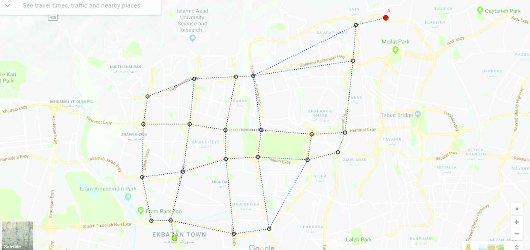
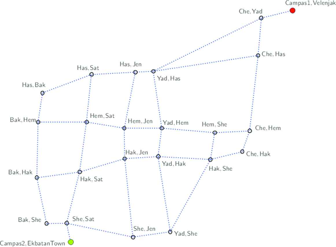
Now, we consider each of the intersections as one vertex and each highways between two intersections as the edge of graph. There are many routes from campus 1 to 2 related to this university. However, the main question raised here is, related to the least time each route requires. In this regard, a lot of parameters may play a role are but the tolerance of traffic and distance between two intersection are considered as two main parameters. Further, the volume of traffic and distance between two intersections are fuzzy variable and interval-valued fuzzy variable, respectively.
Table 5 indicates the data related to the edges based on the reports from traffic and municipal organization in Tehran and daily personal experiences traversing from this route at
Tabular representation of distance and tolerance of traffic.
In order to obtain the best route requiring less time, an algorithm should be first used for finding all the paths from the campus
| i | Paths | Time(H) | i | Paths | Time(H) |
|---|---|---|---|---|---|
| 1 | 0 1 7 8 13 16 17 18 23 | 0.527386364 | 2 | 0 1 7 8 13 12 11 18 23 | 0.534886364 |
| 3 | 0 1 7 8 13 12 17 18 23 | 0.439172078 | 4 | 0 1 7 8 9 10 11 18 23 | 0.481914336 |
| 5 | 0 1 7 8 9 12 11 18 23 | 0.540453297 | 6 | 0 1 7 8 9 12 17 18 23 | 0.415875375 |
| 7 | 0 1 7 14 13 16 17 18 23 | 0.505957792 | 8 | 0 1 7 14 13 12 11 18 23 | 0.567321429 |
| 9 | 0 1 7 14 13 12 17 18 23 | 0.442743506 | 10 | 0 1 7 14 15 16 17 18 23 | 0.414707792 |
| 11 | 0 1 2 3 4 5 10 11 18 23 | 0.476609848 | 12 | 0 1 2 3 6 5 10 11 18 23 | 0.478216991 |
| 13 | 0 1 2 7 8 13 16 17 18 23 | 0.55030303 | 14 | 0 1 2 7 8 13 12 11 18 23 | 0.636666667 |
| 15 | 0 1 2 7 8 13 12 17 18 23 | 0.512088745 | 16 | 0 1 2 7 8 9 10 11 18 23 | 0.554831002 |
| 17 | 0 1 2 7 8 9 12 11 18 23 | 0.613369963 | 18 | 0 1 2 7 8 9 12 17 18 23 | 0.488792041 |
| 19 | 0 1 2 7 14 13 16 17 18 23 | 0.553874459 | 20 | 0 1 2 7 14 13 12 11 18 23 | 0.640238095 |
| 21 | 0 1 2 7 14 13 12 17 18 23 | 0.515660173 | 22 | 0 1 2 7 14 15 16 17 18 23 | 0.487624459 |
| 23 | 0 1 7 8 13 16 17 21 22 18 23 | 0.526475694 | 24 | 0 1 7 8 13 16 20 21 22 18 23 | 0.512586806 |
| 25 | 0 1 7 8 13 12 17 21 22 18 23 | 0.488261409 | 26 | 0 1 7 8 9 12 17 21 22 18 23 | 0.464964705 |
| 27 | 0 1 7 14 13 16 17 21 22 18 23 | 0.530047123 | 28 | 0 1 7 14 13 16 20 21 22 18 23 | 0.516158234 |
| 29 | 0 1 7 14 13 12 17 21 22 18 23 | 0.491832837 | 30 | 0 1 7 14 15 16 17 21 22 18 23 | 0.463797123 |
| 31 | 0 1 7 14 15 16 20 21 22 18 23 | 0.449908234 | 32 | 0 1 7 14 15 19 20 21 22 18 23 | 0.437408234 |
| 33 | 0 1 2 3 4 5 9 10 11 18 23 | 0.558306277 | 34 | 0 1 2 3 4 5 9 12 11 18 23 | 0.616845238 |
| 35 | 0 1 2 3 4 5 9 12 17 18 23 | 0.492267316 | 36 | 0 1 2 3 6 5 9 10 11 18 23 | 0.55991342 |
| 37 | 0 1 2 3 6 5 9 12 11 18 23 | 0.618452381 | 38 | 0 1 2 3 6 5 9 12 17 18 23 | 0.563517316 |
| 39 | 0 1 2 3 6 8 13 12 17 18 23 | 0.53530303 | 40 | 0 1 2 3 6 8 9 10 11 18 23 | 0.578045288 |
| 41 | 0 1 2 3 6 8 9 12 11 18 23 | 0.636584249 | 42 | 0 1 2 3 6 8 9 12 17 18 23 | 0.512006327 |
| 43 | 0 1 2 7 8 13 16 17 21 22 18 23 | 0.599392361 | 44 | 0 1 2 7 8 13 16 20 21 22 18 23 | 0.585503472 |
| 45 | 0 1 2 7 8 13 12 17 21 22 18 23 | 0.561178075 | 46 | 0 1 2 7 8 9 12 17 21 22 18 23 | 0.537881372 |
| 47 | 0 1 2 7 14 13 16 17 21 22 18 23 | 0.60296379 | 48 | 0 1 2 7 14 13 16 20 21 22 18 23 | 0.589074901 |
| 49 | 0 1 2 7 14 13 12 17 21 22 18 23 | 0.564749504 | 50 | 0 1 2 7 14 15 16 17 21 22 18 23 | 0.53671379 |
| 51 | 0 1 2 7 14 15 16 20 21 22 18 23 | 0.522824901 | 52 | 0 1 2 7 14 15 19 20 21 22 18 23 | 0.510324901 |
| 53 | 0 1 2 3 4 5 9 12 17 21 22 18 23 | 0.541356647 | 54 | 0 1 2 3 6 5 9 12 17 21 22 18 23 | 0.54296379 |
| 55 | 0 1 2 3 6 8 13 16 17 21 22 18 23 | 0.622606647 | 56 | 0 1 2 3 6 8 13 16 20 21 22 18 23 | 0.608717758 |
| 57 | 0 1 2 3 6 8 13 12 17 21 22 18 23 | 0.584392361 | 58 | 0 1 2 3 6 8 9 12 17 21 22 18 23 | 0.561095658 |
Tabular representation all paths obtained from C++ program.
Thus, the time of crossing every path is as follows:
Further, as shown in Table 6, we could find the time for any path by using an Algorithm 2 as follows:
Finally, the optimum path spending the least time was evaluated for its crossing. As displayed in Table 6, the optimum path is
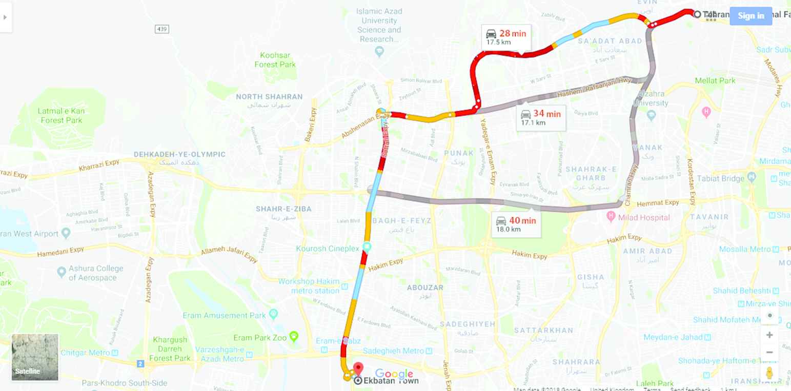
Checking (or Comparing) the accuracy of the algorithm with Google Map software.
5. CONCLUSION
Graph theoretical concepts are widely used to study and model various applications in different areas including automata theory, operations research, economics and transportation. However, in many cases, some aspects of a graph-theoretic problem may be vague or uncertain. Fuzzy graphs were introduced by Rosenfeld [1], ten years after Zadeh's landmark paper “Fuzzy Sets” (briefly
Algorithm 1: Finding all the paths from the campus 1 2
Data: Cubic graph from the campus
Result: Finding all the paths from the campus
1. Define utility function for printing the found path in cubic graph.
2. Define utility function to check if current vertex is already present in cubic path.
3. Define utility function for finding paths in cubic graph from source to destination(int g, int src, int dst, int v).
4. If last vertex is the desired destination then print the cubic path.
5. Traverse to all the nodes connected to current vertex and push new path to queue.
6. The main program.
6.1. The number of vertices with information on them.
6.2. The construct an edge between vertices with information on them.
6.3. Call all of defined utility functions and print the cubic path.
6.4. Return to the initial vertex.
Algorithm 2: Finding the time needs for the crossing of any cubic path
Data: All the cubic paths from the campus
Result: Finding the time needs for the crossing of any cubic path initializations
1. Define function
2. Define function
3. Define function
4. The main program.
Add all of the cubic paths with information on them.
Compare between
Print the cubic paths with time needs for the crossing in Table 6.
| Researchers | Title | Technique Used | Results |
|---|---|---|---|
| Riedel and Brunner [39] | Traffice control using graph theory | The design of a controller for a traffic crossing is presented by means of an example. The controller to be developed has to minimize the waiting time of public transportation while maintaining the individual traffic flowing as well as possible. | The simulation results have shown that it is possible to halve the average waiting time of public transportation while the average waiting time of the cars remains almost unchanged. Problems only raised in the paper:
|
| Firouzian and Nouri Jouybari [40] | Coloring fuzzy graphs and traffic light problem | They introduced the main approach to the fuzzy coloring problem and used in the traffic lights problem. | They tried to model the traffic lights problem at a junction such that to avoid long time waiting at junctions and congestions. |
| Dave and Jhala [41] | Application of graph theory in traffic management | The compatibility graph corresponding to the problem and circular-arc graphs have been introduced. Compatibility graph corresponding to the problem, spanning subgraph and circular-arc graphs then are utilized to reduce our problem to the solution of LP problems. | They tried to solve the problem of the phasing of traffic lights at a junction such that traffic signals can be used more efficiently to avoid a long time waiting at junctions and congestions. |
| Myna [42] | Application of fuzzy graph in traffic | They used a fuzzy graph model to represent a traffic network of a city and discussed a method to find the different types of accidental zones in traffic flows using edge coloring of a fuzzy graph. | They give a speed limit of vehicles according to the accidental zone. The chromatic number of |
| Abdushukoor and Sushama [43] | A fuzzy graph approach for selecting optimal traffic counting locations in road networks | They proposed a methodology, which is designed to handle the situation in which the origin-destination matrix is unavailable or scarce. It requires traffic count data on links and also, presented a methodology for identifying traffic counting locations which uses a screen-line-based approach to cover all paths having a particular flow or higher, in order to attain maximum flow coverage goal. | They presented models for finding (1) the optimum number of traffic counting locations and (2) maximum flow captured by these locations. |
| Setiawan and Budayasa [44] | Application of graph theory concept for traffic light control at crossroad | By modeling the system of traffic flows into a compatible graph, two vertices are represented as the flow connected by an edge if and only if the flow at the crossroads can be moved simultaneously without causing crashes. | The calculation of the optimal cycle states traffic light cycle at different times at crossroads and when the green light in all directions. But in fact, the traffic light settings are very complicated and no single, which involves a variety of factors, and cannot adopt a suitable model to solve all problems. |
| Singh Oberoi et al. [45] | Spatial modeling of urban road traffic using graph theory | They presented a qualitative model, based on graph theory, which will help to understand the spatial evolution of urban road traffic. Various real-world objects which affect the flow of traffic, and the spatial relations between them, are included in the model definition. | They presented their initial ideas to develop a spatial model to understand the urban road traffic using heterogeneous data available at different levels of detail and the idea of categorizing the real-world objects into various classes and associate a specific set of spatial relations to each class. They also proposed two types of granularity: carriageway-based and sector-based. |
| Dey et al. [46] | New concepts on vertex and edge coloring of simple vague graphs | They analyzed the concept of vertex and edge coloring on simple vague graphs and the applications of the proposal in solving practical problems related to traffic flow management and the selection of advertisement spots are mainly discussed. | The applicability and practical aspects of all of the concepts and definitions introduced were demonstrated using two scenarios related to traffic flow and advertising. The edge coloring for vague graphs was used to model traffic light positioning and scheduling to optimize the traffic flow in a town setting, whereas the vertex coloring was used to model a problem involving the selection of the best place for a company to place its advertisement. |
| Satyanarayana [38] | Range-valued fuzzy coloring of interval-valued fuzzy graphs | He introduced coloring interval-valued fuzzy graphs that have a few general applications and also another idea of using coloring for interval-valued fuzzy graphs is presented. This procedure is utilized to color the India political map, revealing the power of the relationship within the nation. Additionally, another sort of traffic signal system is analyzed. | Interval-valued fuzzy graphs appropriately signify a few public problems. One is the India political map. The current maps do not give information on the political connection among neighboring nations. However, the interval-valued fuzzy graph gives a genuine picture of the political connections. This introduced the coloring of interval-valued fuzzy graphs and showed the political connection among the nations. In addition, straight traffic signals, red, green, and so on, do not suitably represent traffic systems. Hence, range-valued fuzzy colors are used to simplify the available systems. Thus, the traffic signal problem is explained here by coloring interval-valued fuzzy graphs. Branch coloring is also significant for some genuine events. We are working on the branch coloring and total coloring of interval-valued fuzzy graphs as an added layer of this subject. |
As you see in the above report, more than 90 percent of researchers did use the graph theory and fuzzy graph theory in traffic flows. In fact, they studied a limited branch of traffic problems as follows:
Optimization of traffic light's function
Evaluation traffic by image processing
Identification high-risk areas on urban roads and optimization of the urban road traffic
None researchers not used graph theory, fuzzy graph theory and, etc., for finding the best path from the origin to the destination. Therefore, we tried to find the best path from the origin to the destination by using graph theory, fuzzy graph theory and, etc. It is natural to deal with the vagueness and uncertainty using the methods of fuzzy graphs and interval-valued fuzzy graphs in some problems. Thus, Jun et al. introduced a cubic set that is combined by a fuzzy set and interval-valued fuzzy set. A cubic model is a generalized form of a fuzzy model and an interval-valued fuzzy model. In our goal, the cubic models provide more precision, flexibility and compatibility to the system when more than one agreements are to be dealt with. Thus in this article, we introduced a cubic graph and we know that the notion of the cubic graph which is different from the cubic graph in [18] is introduced, and many properties are considered. The cubic graph has found its importance as a closer approximation to real-life situations. The detailed study on the soft cubic graphs on to find one path with the minimum distance in minimum time, if there exist some problems in the path of one address is one of the primary focus of our future research work. For future works, we will the study of cubic graphs may also be extended with an application of cubic graph in neural networks, data science and medical science. The proposed concepts can be used in communication systems, image processing, system analysis and pattern recognition, etc.
CONFLICT OF INTEREST
This manuscript has not been submitted to, nor is under review at, another journal or other publishing venue.
AUTHORS' CONTRIBUTIONS
All authors have participated in (a) conception and design, or analysis and interpretation of the data; (b) drafting the article or revising it critically for important intellectual content; and (c) approval of the final version.
Funding Statement
The authors have no affiliation with any organization with a direct or indirect financial interest in the subject matter discussed in the manuscript.
ACKNOWLEDGMENTS
The authors are very indebted to the editor and anonymous referees for their careful reading and valuable suggestions which helped to improve the readability of the paper.
REFERENCES
Cite this article
TY  - JOUR
AU  - G. Muhiuddin
AU  - M. Mohseni Takallo
AU  - Y. B. Jun
AU  - R. A. Borzooei
PY  - 2020
DA  - 2020/08/18
TI  - Cubic Graphs and Their Application to a Traffic Flow Problem
JO  - International Journal of Computational Intelligence Systems
SP  - 1265
EP  - 1280
VL  - 13
IS  - 1
SN  - 1875-6883
UR  - https://doi.org/10.2991/ijcis.d.200730.002
DO  - 10.2991/ijcis.d.200730.002
ID  - Muhiuddin2020
ER  -