
A Novel Two-Stage DEA Model in Fuzzy Environment: Application to Industrial Workshops Performance Measurement
 , F. Movahhedi Sobhani1, S. E. Najafi1
- DOI
- 10.2991/ijcis.d.200731.002How to use a DOI?
- Keywords
- Efficiency; Fuzzy data envelopment analysis; Two-stage DEA model; Industrial workshops
- Abstract
One of the paramount mathematical methods to compute the general performance of organizations is data envelopment analysis (DEA). Nevertheless, in some cases, the decision-making units (DMUs) have middle values. Furthermore, the conventional DEA models have been originally formulated solely for crisp data and cannot handle the problems with uncertain information. To tackle the above issues, this paper presents a two-stage DEA model with fuzzy data. The recommended technique is based on the fuzzy arithmetic and has a simple construction. Furthermore, to illustrate the new model, we investigate the efficiency of some industrial workshops in Iran. The results show the effectiveness and robustness of the new model.
- Copyright
- © 2020 The Authors. Published by Atlantis Press B.V.
- Open Access
- This is an open access article distributed under the CC BY-NC 4.0 license (http://creativecommons.org/licenses/by-nc/4.0/).
1. INTRODUCTION
Data envelopment analysis (DEA) is a linear programming approach for evaluating relative efficiency or calculating the efficiency of the finite number of similar decision-making units (DMUs), which has multiple inputs and outputs [1]. Three popular models of DEA have been proposed. The first model presented in the DEA is the Charnes-Cooper-Rhodes model (CCR) model and was introduced by Charnes, Chopper and Rohdes in 1978 [1]. Banker, Charnes and Chopper introduced the new model, with the change in the CCR model and to solve its problem, which was named BCC according to the first letters of their last name and the third popular DEA model is the additive model [2].
In recent years, studies have been done on the two-stage data arrangement. Along with the inputs and outputs, we also have a set of “middle values (intermediate)” which is between these two stages. The middle values are outputs of the first stage and used as inputs in the second stage. Kao and Hwang [3] established a type of this model that deliberated the series connection of the sub-processes and applied this model for the Taiwanese nonlife insurance companies. Chen et al. [4] with a weighted sum of the efficiencies of the two distinct stages modelled the efficiency of a two-stage process. Wang and Chin [5] modelled the overall efficiency of the two-stage process as a weighted harmonic measure of the efficiencies of two individual stages, which expanded it by assuming the return on a variable scale. Forghani and Najafi [6], applied the sensitivity analysis to DMUs for two-stage DEA. Furthermore, in recent years, numerous reports and articles have been published in esteemed global journals verifying that two-stage DEA is operational; see [7,8,9,10,11,12,13,14].
However, in some cases, the values of the data are often information with indeterminacy, impreciseness, vagueness, inconsistent and incompleteness. Inaccurate assessments are mainly the outcome of information that is unquantifiable, incomplete and unavailable. Data in the conventional models of DEA are certain; nevertheless, there are abundant situations in actuality where we have to face uncertain restrictions. Therefore, by considering the gray dimension in the classical logic that is the same fuzzy logic, the results obtained in DEA models can be improved. Zadeh first anticipated the fuzzy sets (FSs) in contradiction of certain logic and at the time, his primary goal was to develop a more efficient model for describing the process of natural linguistic terms processing [15]. After this work, numerous scholars considered this topic; see [16–27].
Khalili-Damghani et al. [28] proposed a fuzzy two-stage data envelopment analysis model (FTSDEA) to calculate the efficiency score of each DMU and sub-DMU. The proposed model was linear and independent of its α-cut variables. Khalili-Damghani and Taghavifard [29] also proposed the sensitivity analysis in fuzzy two-stage DEA models. Beigi and Gholami proposed a model to estimate the efficiency score fuzzy two-stage DEA and suggested a model to allocate resources [30]. Tavana and Khalili-Damghani [31] using the Stackelberg game approach proposed an efficient two-stage fuzzy DEA model to calculate the efficiency scores for a DMU and its sub-DMUs. Nabahat [32] presented a fuzzy version of a two-stage DEA model with a symmetrical triangular fuzzy number. The basic idea is to transform the fuzzy model into crisp linear programming by using the α-cut approach. Zhou et al. [33] proposed undesirable two-stage fuzzy DEA models to estimate the efficiency of banking system. This system is divided into production and profit sub-systems. They proposed the model with two assumptions of constant returns-to-scale (CRS) and variable returns-to-scale (VRS), and fuzzy parameters are adopted to describe the uncertain factors. They illustrate and validate the proposed models by evaluating 16 Chinese commercial banks; see also [33–39]. Therefore, there is still a need from the fuzzy two-stage DEA method to develop a new model that keeps original advantage and easy in implementations.
Consequently, in this study, we establish a novel two-stage DEA model in which all data are fuzzy. Furthermore, a competent algorithm for solving the new DEA model has been presented. The main contributions of this paper are three fold: we (1) present a new model of FTSDEA for calculating the efficiency interval with the help of the α-cut for two-stage issues; (2) we also adapt the Wang and Chin model [5] incorporating fuzzy data/values; (3) A real-world case study, considering data from industrial workshops, is employed to illustrate the application, by means of the proposed algorithm to compute the efficiency of the resulting DMUs.
The paper unfolds as follows: some basic knowledge and concepts on FSs are deliberated in Section 2. In Section 3, we review the two-stage DEA method of Wang and Chin [5] to calculate the CRS efficiency scores. In Section 4, according to the crisp model of Wang and Chin [5], a new two-stage DEA model has been presented with fuzzy data. Also by using α-cut technique, the original (main) problem has been converted into linear programming. In Section 5, the proposed model and the related algorithm are illustrated with some industrial workshops to ensure their validity and usefulness over the existing models. Finally, conclusions are offered in Section 6.
2. CONCEPTS AND PREREQUISITES
Here, we will discuss some basic definitions related to FSs and trapezoidal fuzzy numbers (TrFNs), respectively [20,31,40].
Definition 2.1.
[40] Let X be a nonempty set, and
Definition 2.2.
[31] For
Definition 2.3.
[31] A fuzzy number
3. TWO-STAGE MODEL OF WANG AND CHIN
In this section, we review the two-stage DEA method of Wang and Chin [5] to calculate the constant return to scale (CRS) efficiency scores. Then a new two-stage fuzzy model has been suggested based on this model. Suppose that, there are n DMUs and that each DMUq
Then the overall efficiency with CRS in the Wang and Chin models is as follows:
S.t
Some definitions of the variables used in the model are as follows:
The first stage efficiency with CRS in the Wang and Chin models is [5]
S.t
The second stage efficiency with CRS in the Wang and Chin models is as follows:
S.t
4. THE PROPOSED TWO-STAGE FUZZY DEA MODEL
Consider the TrFN in the left and right spread format as inputs, intermediate measures and outputs of n DMUs with two-stage processes. Each DMUq
The upper
S.t
The Model (14) is a nonlinear mathematical programming model and its global optimum cannot be found easily. Moreover, Model (14) is dependent on the α-cut and should be solved for different α-cut levels with a predetermined step-size. The values of Equations (8–13) has been replaced in Model (14):
S.t
In Model (15), the input variables take lower bound and output variables take upper bound for DMU under consideration as well as its associated sub-DMUs. For all other DMUs and sub-DMUs, the input variables take upper bound and output variables take lower bound. So, Model (15) yields the upper bound of overall efficiency
S.t
Similarly we get
S.t
Let us consider
Replacement of (18) to (23) in the Model (15) we will obtain the Model (24).
S.t
The Model (24) is always feasible because it satisfies all the constraints in Model (24) and it is independent of the inputs, intermediate measures, outputs and the α-cut level values. Accordingly, the efficiency of the model is equal to the optimal value, in the sense that e is equal to 1 in the best possible way.
Also, by replacement of (18) to (23) in Model (17) we will obtain the Model (25):
S.t
This model is also always feasible, like the Model (24). In addition, Models of (24) and (25) are linear programming problems. The Models (24) and (25) have been developed based on optimistic and pessimistic situations. The optimal values of
4.1. Maximum Achievable Value of the Efficiency for the Sub-DMU in the First Stage
Applying the same procedure on the Model (6), we obtain the Model (26) and the Model (28) which can measure the optimistic and pessimistic values of maximum achievable efficiency of the first stage.
4.1.1. Upper bound in the first stage
S.t
We calculated the value of
This solution is always feasible, like the Model (24).
4.1.2. Lower bound in the first stage
S.t
We calculate the value of
This solution is always feasible, like the model (24).
In models (26) and (28), we calculated the
4.2. Maximum Achievable Value of the Efficiency for the Sub-DMU in the Second Stage
Alternatively, applying the same procedure in the previous models on Model (7), we obtain the Model (30) and the Model (31) which can measure the optimistic and pessimistic values of maximum achievable efficiency of the second stage.
4.2.1. Upper bound in the second stage
S.t
This solution is always feasible, like the Model (24).
4.2.2. Lower bound in the second stage
S.t
This solution is always feasible like the model (24).
The overall efficiency is obtained from the following formula:
The values
The values of
5. NUMERICAL EXAMPLE
This paper aimed to use the fuzzy two-stage DEA technique for efficiency measurement. So in this paper, the proposed model is used to determine the efficiency of industrial workshops of 10–49 personnel in Iran in 2014. In this section, the results of the solution of these models are presented, and the efficiency and inefficiency of each unit will be shown. Also, GAMS software is used for calculation (computing).
5.1. Define the Levels of Two-Stage DEA for the Example
In this paper, we separated the two-stage process into two parts: production and sales. Production: in the production part, all the ingredients and materials are needed to produce the product and also the final output is the first stage of our method. Sale: the value of the output obtained in the production part and the amount (value) of income from the activities performed are examined; see the Figure 1. Since, in this paper, industrial workshops are our DMUs, this problem can be divided into two parts. The first part is based on the province and the second part is based on the essential activity of the industrial workshops. The results of the efficiency of industrial workshops are shown in Tables 1–6 (see also Appendix).
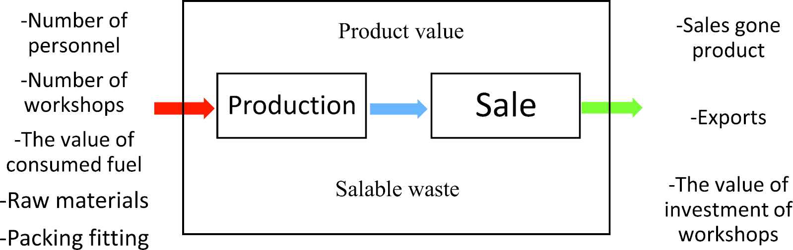
Two-stage Data envelopment analysis (DEA) process.
| Row | Province | Upper Bound | Lower Bound | Efficiency | Rank | ||
|---|---|---|---|---|---|---|---|
| 1 | Whole country | 0.8345 | 0.6141 | 0.5833 | 0.4167 | 0.7427 | 13 |
| 2 | East Azerbaijan | 0.8207 | 0.6191 | 0.5800 | 0.4200 | 0.7360 | 21 |
| 3 | West Azerbaijan | 0.8470 | 0.6242 | 0.5845 | 0.4155 | 0.7544 | 9 |
| 4 | Ardabil | 0.8239 | 0.6213 | 0.5812 | 0.4188 | 0.7391 | 17 |
| 5 | Isfahan | 0.8232 | 0.6208 | 0.5809 | 0.4191 | 0.7384 | 18 |
| 6 | Alborz | 0.7995 | 0.6593 | 0.5441 | 0.4559 | 0.7356 | 22 |
| 7 | ILam | 0.8459 | 0.6355 | 0.5846 | 0.4154 | 0.7585 | 6 |
| 8 | Bushehr | 0.8000 | 0.6183 | 0.5804 | 0.4196 | 0.7238 | 28 |
| 9 | Tehran | 0.8249 | 0.6218 | 0.5817 | 0.4183 | 0.7399 | 16 |
| 10 | Charmaholo Bakhtiyari | 0.8200 | 0.6300 | 0.5806 | 0.4194 | 0.7403 | 15 |
| 11 | South Khorasan | 0.7962 | 0.6148 | 0.5775 | 0.4225 | 0.7196 | 31 |
| 12 | Khorasan Razavi | 0.8475 | 0.6358 | 0.5866 | 0.4134 | 0.7600 | 4 |
| 13 | North Khorasan | 0.8715 | 0.6200 | 0.6102 | 0.3898 | 0.7735 | 2 |
| 14 | Khuzestan | 0.7986 | 0.6177 | 0.5790 | 0.4210 | 0.7224 | 29 |
| 15 | Zanjan | 0.7970 | 0.6167 | 0.5781 | 0.4219 | 0.7209 | 30 |
| 16 | Semnan | 0.7994 | 0.6477 | 0.5615 | 0.4385 | 0.7329 | 23 |
| 17 | Sistano Baluchestan | 0.7967 | 0.6260 | 0.5781 | 0.4219 | 0.7247 | 27 |
| 18 | Fars | 0.7956 | 0.5953 | 0.5968 | 0.4032 | 0.7148 | 32 |
| 19 | Qazvin | 0.8452 | 0.6345 | 0.5841 | 0.4159 | 0.7576 | 7 |
| 20 | Qom | 0.8207 | 0.6198 | 0.5806 | 0.4194 | 0.7364 | 20 |
| 21 | Kurdistan | 0.8450 | 0.6146 | 0.5833 | 0.4167 | 0.7490 | 12 |
| 22 | Kerman | 0.8217 | 0.6200 | 0.5806 | 0.4194 | 0.7371 | 19 |
| 23 | Kermanshah | 0.7985 | 0.6270 | 0.5788 | 0.4212 | 0.7263 | 26 |
| 24 | Khogeluye va BoyerAhmad | 0.7979 | 0.6475 | 0.5606 | 0.4394 | 0.7318 | 24 |
| 25 | Golestan | 0.8700 | 0.6200 | 0.6071 | 0.3929 | 0.7718 | 3 |
| 26 | Gilan | 0.8435 | 0.6242 | 0.5824 | 0.4176 | 0.7519 | 11 |
| 27 | Lorestan | 0.8212 | 0.6305 | 0.5816 | 0.4184 | 0.7414 | 14 |
| 28 | Mazandaran | 0.8450 | 0.6242 | 0.5833 | 0.4167 | 0.7530 | 10 |
| 29 | Markazi | 0.8465 | 0.6356 | 0.5850 | 0.4150 | 0.7590 | 5 |
| 30 | Hormozgan | 0.8975 | 0.5875 | 0.6346 | 0.3654 | 0.7842 | 1 |
| 31 | Hamedan | 0.8445 | 0.6345 | 0.5833 | 0.4167 | 0.7570 | 8 |
| 32 | Yazd | 0.7984 | 0.6379 | 0.5606 | 0.4394 | 0.7279 | 25 |
The final output based on the province and
| Row | Activity | Upper Bound | Lower Bound | Efficiency | Rank | ||
|---|---|---|---|---|---|---|---|
| 1 | Whole industry | 0.8190 | 0.6088 | 0.5792 | 0.4208 | 0.7305 | 8 |
| 2 | Food and potable industries | 0.7984 | 0.6135 | 0.5752 | 0.4248 | 0.7199 | 21 |
| 3 | Production of textiles | 0.8237 | 0.6230 | 0.5831 | 0.4169 | 0.7400 | 3 |
| 4 | Clothing production | 0.8185 | 0.5870 | 0.6207 | 0.3793 | 0.7307 | 7 |
| 5 | Tanning and handling leather | 0.8446 | 0.6130 | 0.6034 | 0.3966 | 0.7527 | 2 |
| 6 | Production of wood and wood products | 0.8000 | 0.6367 | 0.5617 | 0.4383 | 0.7284 | 10 |
| 7 | Production of paper and paper products | 0.7975 | 0.5925 | 0.5968 | 0.4032 | 0.7148 | 23 |
| 8 | Spread and print and increase recorded media | 0.8992 | 0.6056 | 0.6346 | 0.3654 | 0.7919 | 1 |
| 9 | Coal refinery petroleum production industries | 0.7995 | 0.6365 | 0.5606 | 0.4394 | 0.7279 | 11 |
| 10 | Industries of materials and chemical products | 0.7986 | 0.6234 | 0.5781 | 0.4219 | 0.7247 | 15 |
| 11 | Production of rubber and plastic products | 0.7976 | 0.6223 | 0.5760 | 0.4240 | 0.7233 | 17 |
| 12 | Production of other nonmetallic minerals | 0.7988 | 0.6332 | 0.5791 | 0.4209 | 0.7291 | 9 |
| 13 | Essential metals production | 0.7971 | 0.6221 | 0.5781 | 0.4219 | 0.7226 | 18 |
| 14 | Production of fabricated metal products | 0.7989 | 0.6141 | 0.5781 | 0.4219 | 0.7209 | 20 |
| 15 | Production of unclassified machinery and equipment | 0.8003 | 0.6250 | 0.5808 | 0.4192 | 0.7268 | 12 |
| 16 | Production of administrative and calculator machines | 0.7950 | 0.6050 | 0.5968 | 0.4032 | 0.7184 | 22 |
| 17 | Production of generating machinery and electricity transmission | 0.7983 | 0.6229 | 0.5765 | 0.4235 | 0.7240 | 16 |
| 18 | Production of radio and television and communication machine | 0.7950 | 0.6141 | 0.5960 | 0.4040 | 0.7219 | 19 |
| 19 | Production of medical tool | 0.7996 | 0.6249 | 0.5794 | 0.4206 | 0.7261 | 13 |
| 20 | Production of motor transport, trailers and semi-trailers | 0.8207 | 0.6198 | 0.5806 | 0.4194 | 0.7364 | 4 |
| 21 | Production of other transport equipment | 0.7992 | 0.6240 | 0.5788 | 0.4212 | 0.7254 | 14 |
| 22 | Furniture production | 0.8195 | 0.6186 | 0.5794 | 0.4206 | 0.7350 | 5 |
| 23 | Salvage (recover) | 0.8001 | 0.6447 | 0.5606 | 0.4394 | 0.7318 | 6 |
The final output based on the industrial workshops and
| Row | Province | Upper Bound | Lower Bound | Efficiency | Rank | ||
|---|---|---|---|---|---|---|---|
| 1 | Whole country | 0.8446 | 0.2945 | 0.6894 | 0.3106 | 0.6737 | 15 |
| 2 | East Azerbaijan | 0.8432 | 0.3216 | 0.6791 | 0.3209 | 0.6758 | 13 |
| 3 | West Azerbaijan | 0.8608 | 0.3207 | 0.6846 | 0.3154 | 0.6905 | 5 |
| 4 | Ardabil | 0.8344 | 0.2937 | 0.6866 | 0.3134 | 0.6649 | 21 |
| 5 | Isfahan | 0.8349 | 0.2942 | 0.6866 | 0.3134 | 0.6654 | 20 |
| 6 | Alborz | 0.8182 | 0.3471 | 0.6438 | 0.3562 | 0.6504 | 30 |
| 7 | ILam | 0.8537 | 0.3125 | 0.6818 | 0.3182 | 0.6815 | 8 |
| 8 | Bushehr | 0.8258 | 0.3058 | 0.6739 | 0.3261 | 0.6562 | 26 |
| 9 | Tehran | 0.8432 | 0.3030 | 0.6791 | 0.3209 | 0.6698 | 17 |
| 10 | Charmaholo Bakhtiyari | 0.8357 | 0.3139 | 0.6765 | 0.3235 | 0.6669 | 18 |
| 11 | South Khorasan | 0.8248 | 0.3048 | 0.6739 | 0.3261 | 0.6552 | 27 |
| 12 | Khorasan Razavi | 0.8502 | 0.3090 | 0.6818 | 0.3182 | 0.6780 | 12 |
| 13 | North Khorasan | 0.8803 | 0.3074 | 0.7016 | 0.2984 | 0.7093 | 2 |
| 14 | Khuzestan | 0.8268 | 0.3068 | 0.6739 | 0.3261 | 0.6572 | 25 |
| 15 | Zanjan | 0.8344 | 0.3242 | 0.6667 | 0.3333 | 0.6644 | 23 |
| 16 | Semnan | 0.8195 | 0.3395 | 0.6528 | 0.3472 | 0.6528 | 28 |
| 17 | Sistano Baluchestan | 0.8284 | 0.3204 | 0.6643 | 0.3357 | 0.6579 | 24 |
| 18 | Fars | 0.8346 | 0.2923 | 0.6866 | 0.3134 | 66460 | 22 |
| 19 | Qazvin | 0.8517 | 0.3105 | 0.6818 | 0.3182 | 67950 | 11 |
| 20 | Qom | 0.8432 | 0.3123 | 0.6791 | 0.3209 | 67280 | 16 |
| 21 | Kurdistan | 0.8611 | 0.3098 | 0.6953 | 0.3047 | 69310 | 4 |
| 22 | Kerman | 0.8444 | 0.3135 | 0.6791 | 0.3209 | 67400 | 14 |
| 23 | Kermanshah | 0.8186 | 0.3046 | 0.6714 | 0.3286 | 64970 | 31 |
| 24 | Khogeluye va BoyerAhmad | 0.8217 | 0.3296 | 0.6528 | 0.3472 | 65080 | 29 |
| 25 | Golestan | 0.8700 | 0.3000 | 0.7097 | 0.2903 | 70450 | 3 |
| 26 | Gilan | 0.8611 | 0.3103 | 0.6846 | 0.3154 | 68740 | 6 |
| 27 | Lorestan | 0.8314 | 0.3198 | 0.6765 | 0.3235 | 66590 | 19 |
| 28 | Mazandaran | 0.8520 | 0.3010 | 0.6923 | 0.3077 | 68250 | 7 |
| 29 | Markazi | 0.8522 | 0.3110 | 0.6818 | 0.3182 | 68000 | 10 |
| 30 | Hormozgan | 0.9100 | 0.2900 | 0.7500 | 0.2500 | 75500 | 1 |
| 31 | Hamedan | 0.8532 | 0.3120 | 0.6818 | 0.3182 | 68100 | 9 |
| 32 | Yazd | 0.8172 | 0.3184 | 0.6620 | 0.3380 | 64860 | 32 |
The final output of the method [28] based on the province and
| Row | Activity | Upper Bound | Lower Bound | Efficiency | Rank | ||
|---|---|---|---|---|---|---|---|
| 1 | Whole industry | 0.8366 | 0.2949 | 0.6791 | 0.3209 | 0.6628 | 8 |
| 2 | Food and potable industries | 0.8247 | 0.3050 | 0.6739 | 0.3261 | 0.6552 | 14 |
| 3 | Production of textiles | 0.8444 | 0.3135 | 0.6791 | 0.3209 | 0.6740 | 5 |
| 4 | Clothing production | 0.8429 | 0.2626 | 0.7109 | 0.2891 | 0.6751 | 3 |
| 5 | Tanning and handling leather | 0.8516 | 0.2820 | 0.7031 | 0.2969 | 0.6825 | 2 |
| 6 | Production of wood and wood products | 0.8264 | 0.3352 | 0.6549 | 0.3451 | 0.6569 | 12 |
| 7 | Production of paper and paper products | 0.8344 | 0.2937 | 0.6866 | 0.3134 | 0.6649 | 7 |
| 8 | Spread and print and increase recorded media | 0.8996 | 0.2882 | 0.7328 | 0.2672 | 0.7362 | 1 |
| 9 | Coal refinery petroleum production industries | 0.8256 | 0.3457 | 0.6549 | 0.3451 | 0.6600 | 9 |
| 10 | Industries of materials and chemical products | 0.8248 | 0.3307 | 0.6643 | 0.3357 | 0.6589 | 10 |
| 11 | Production of rubber and plastic products | 0.8252 | 0.3171 | 0.6643 | 0.3357 | 0.6549 | 16 |
| 12 | Production of other nonmetallic minerals | 0.8172 | 0.3184 | 0.6620 | 0.3380 | 0.6486 | 20 |
| 13 | Essential metals production | 0.8254 | 0.3174 | 0.6643 | 0.3357 | 0.6549 | 15 |
| 14 | Production of fabricated metal products | 0.8257 | 0.3060 | 0.6739 | 0.3261 | 0.6562 | 13 |
| 15 | Production of unclassified machinery and equipment | 0.8237 | 0.3297 | 0.6643 | 0.3357 | 0.6579 | 11 |
| 16 | Production of administrative and calculator machines | 0.8181 | 0.2576 | 0.6912 | 0.3088 | 0.6450 | 23 |
| 17 | Production of generating machinery and electricity transmission | 0.8241 | 0.3162 | 0.6643 | 0.3357 | 0.6536 | 17 |
| 18 | Production of radio and television and communication machine | 0.8179 | 0.2863 | 0.6812 | 0.3188 | 0.6484 | 21 |
| 19 | Production of medical tool | 0.8187 | 0.2957 | 0.6714 | 0.3286 | 0.6468 | 22 |
| 20 | Production of motor transport, trailers and semi-trailers | 0.8450 | 0.3141 | 0.6791 | 0.3209 | 0.6746 | 4 |
| 21 | Production of other transport equipment | 0.8230 | 0.3154 | 0.6643 | 0.3357 | 0.6526 | 18 |
| 22 | Furniture production | 0.8432 | 0.3123 | 0.6791 | 0.3209 | 0.6728 | 6 |
The final output of the method of [28] based on the industrial workshops and
| The Average Efficiency/Methods | The Method of [28] | The Proposed Method |
|---|---|---|
| The efficiency in the first stage | 0.9266 | 1 |
| The efficiency in the second stage | 0.8087 | 0.8747 |
| The final efficiency | 0.6737 | 0.7427 |
The comparison of the efficiency of two methods based on the province.
| The Average Efficiency/Methods | The Method of [28] | The Proposed Method |
|---|---|---|
| The efficiency in the first stage | 0.9383 | 1 |
| The efficiency in the second stage | 0.7978 | 0.8630 |
| The final efficiency | 0.6628 | 0.7305 |
The comparison of the efficiency of two methods based on the industrial workshops.
According to the results, it was determined that none of the provinces are efficient in this model. The same applies to activities. It should be noted that the results are expressed in three parts of the final efficiency, the efficiency of the first stage and the efficiency of the second stage. For the provinces, we have the following results:
The efficiency of the first stage (manufacturing sector): Hormozgan with the efficiency 1, Ardebil with the efficiency 1 and Isfahan with the efficiency of 1 ranked first to third, respectively.
The efficiency of the second stage (sales sector): Hormozgan with the efficiency of 0.9168, North Khorasan with the efficiency of 0.9045 and Golestan with the efficiency of 0.9041 have first to the third rank, respectively.
Final efficiency: Hormozgan, with the efficiency of 0.7842, North Khorasan with the efficiency of 0.7735 and Golestan with the efficiency of 0.7718, ranks first to third, respectively.
If we want to consider the efficiency of the first stage, which is the manufacturing sector, we observe that all DMUs are efficient. In the second stage, which is the sales sector, we observe that none of the DMUs are efficient and the Hormozgan, North Khorasan and Golestan provinces have the highest performance. Now, we present the results at different levels based on the type of workshop activity:
The efficiency of the first stage (manufacturing sector): The clothing production with the efficiency of 1, tanning and handling leather with the efficiency of 1 and the production of radio and television and communication machine with the efficiency of 1, ranks first to third, respectively.
The efficiency of the second stage (sales sector): The spread and print and increase recorded media with the efficiency of 0.9245, tanning and handling leather with the efficiency of 0.8852 and the production of motor transport, trailers and semi-trailers with the efficiency of 0.8706, ranks first to third, respectively.
Final efficiency: The spread and print and increase recorded media with the efficiency of 0.7919, tanning and handling leather with the efficiency of 0.7527and production of textiles with the efficiency of 0.7400, ranks first to third, respectively.
Next, we run the models of [29] and for comparison with our models, the formulas (33) and (34) are used. It should be noted that the ranking of the DMUs whose efficiency was one was used by the L1-norm method proposed in [42]. The results of the efficiency of industrial workshops are shown in the following tables (see also Appendix).
In the following, we compare the average efficiency of the method [29] and the proposed model. Based on Tables 3–4, we have the results of Tables 5 and 6.
By comparing the results of the proposed model with the method of [28], it was found that the score of the efficiency of our method is about 0.0700 higher than the method of [28]. Furthermore, none of the stages of the method [28] are efficient. However, in the second stage of our method, all DMUs are efficient. In the proposed method, we use the weighted average of the outputs of the first and second stages to obtain the final efficiency, while in the method of [28] for obtaining the final efficiency, only the output of the second stage is considered. For this reason, it can be seen that the efficiency obtained by these two models is different and the efficiency scores of the proposed model are slightly higher than the method of [28]. Regarding the inefficiency of the workshops, if we want to study the two-stage study independently and separately, we conclude that all industrial workshops in the manufacturing sector, which is the first stage of our model are efficient. Therefore, the production sector of all these industrial workshops is in excellent condition, and there is no need to improve their performance. However, in the second stage of the research, which is the sale of industrial workshops, all industrial workshops are inefficient, and the workshops do not perform well in this part, and they need to improve their performance. Therefore, according to the results, we conclude that industrial workshops should improve their sales performance by using their facilities as well as marketing, advertising, positive changes on their products and paying attention to the needs of customers as possible, increase the efficiency of their sales and reach the desired level.
6. CONCLUSION
The classical DEA models view DMUs as “black boxes” that consume a set of inputs to produce a set of outputs, and they do not take into consideration the intermediate measures within a DMU. In this paper, a new two-stage fuzzy model was introduced for DEA and efficiency scores were divided into two stages, the lower and upper bounds of the efficiency scores were calculated using the proposed two-stage fuzzy DEA method. Then, for model reliability measurement, the efficiency of industrial workshops between 10 and 49 employees was investigated, and its results were defined in tables.
The contents of the tables and the studies carried out by the proposed model showed that these industrial workshops were inefficient. Since this paper uses the FTSDEA technique, workshops were tested in two stages, which the first stage is production and the second stage is the sale of workshops. The source of this inefficiency can be examined in the first or second stage. As the efficiency scores in the first stage for all units is 1, it can be concluded that the source of changes in the efficiency scores for DMUs is not the first stage. This means that the inefficient source of DMUs can be found in the second stage. This information is used to conclude that the lower and upper bounds of the overall efficiency of the units were less than 1. In the first stage, the upper and lower bounds of the efficiency score of all units were equal to 1. In the second stage, the efficiency score of all DMUs was less than 1. Briefly, the efficiency score in the second stage was less than the efficiency score in the first stage for all units in the industrial workshops. In other words, units generally did not succeed in converting their inputs (sources) into outputs. That is, the source of this inefficiency is inappropriate execution in the second stage for all units.
It is worth mentioning that the uncertainty, ambiguity and indeterminacy in this paper is limited to TrFNs. Nevertheless, the other types of fuzzy numbers such as bipolar FSs and interval-valued fuzzy numbers, Pythagorean FS, q-rung orthopair FS, neutrosophic sets, and so on can also be used to indicate variables characterizing the core in worldwide problems. As for future research, we intend to extend the proposed approach to these kinds of tools.
CONFLICT OF INTEREST
The authors declare that they have no competing interests.
AUTHORS' CONTRIBUTIONS
The study was conceived and designed by M. R. Soltani and S. A. Edalatpanah; also experiments performed by F. Movahhedi Sobhani, and S. E. Najafi. All authors read and approved the manuscript.
Funding Statement
This research received no external funding.
ACKNOWLEDGMENTS
The authors are most grateful to the two anonymous referees for the very constructive criticism on a previous version of this work, which greatly improved the quality of the present paper.
APPENDIX A. LIST OF ACRONYMS
DEA: Data Envelopment Analysis
DMU: Decision-Making Units
CCR model: Charnes, Cooper, Rhodes model
BCC model: Banker, Charnes, Cooper model
CRS: Constant Returns-to-Scale
VRS: Variable Returns-to-Scale
FS: Fuzzy Set
FTSDEA: Fuzzy Two-Stage Data Envelopment Analysis
APPENDIX
| Row | Province | Upper Bound | Lower Bound | W1 | W2 | Efficiency |
|---|---|---|---|---|---|---|
| 1 | Whole country | 1 | 1 | 0.7195 | 0.2805 | 1 |
| 2 | East Azerbaijan | 1 | 1 | 0.6818 | 0.3182 | 1 |
| 3 | West Azerbaijan | 1 | 1 | 0.6955 | 0.3045 | 1 |
| 4 | Ardabil | 1 | 1 | 0.7456 | 0.2544 | 1 |
| 5 | Isfahan | 1 | 1 | 0.7394 | 0.2606 | 1 |
| 6 | Alborz | 1 | 1 | 0.6458 | 0.3542 | 1 |
| 7 | ILam | 1 | 1 | 0.6793 | 0.3207 | 1 |
| 8 | Bushehr | 1 | 1 | 0.7350 | 0.2650 | 1 |
| 9 | Tehran | 1 | 1 | 0.7220 | 0.2780 | 1 |
| 10 | Charmaholo Bakhtiyari | 1 | 1 | 0.7121 | 0.2879 | 1 |
| 11 | South Khorasan | 1 | 1 | 0.7838 | 0.2162 | 1 |
| 12 | Khorasan Razavi | 1 | 1 | 0.7184 | 0.2816 | 1 |
| 13 | North Khorasan | 1 | 1 | 0.7079 | 0.2921 | 1 |
| 14 | Khuzestan | 1 | 1 | 0.7436 | 0.2564 | 1 |
| 15 | Zanjan | 1 | 1 | 0.6977 | 0.3023 | 1 |
| 16 | Semnan | 1 | 1 | 0.6769 | 0.3231 | 1 |
| 17 | Sistano Baluchestan | 1 | 1 | 0.7100 | 0.2900 | 1 |
| 18 | Fars | 1 | 1 | 0.7917 | 0.2083 | 1 |
| 19 | Qazvin | 1 | 1 | 0.7155 | 0.2845 | 1 |
| 20 | Qom | 1 | 1 | 0.6778 | 0.3222 | 1 |
| 21 | Kurdistan | 1 | 1 | 0.7036 | 0.2964 | 1 |
| 22 | Kerman | 1 | 1 | 0.6988 | 0.3012 | 1 |
| 23 | Kermanshah | 1 | 1 | 0.7375 | 0.2625 | 1 |
| 24 | Khogeluye va BoyerAhmad | 1 | 1 | 0.6758 | 0.3242 | 1 |
| 25 | Golestan | 1 | 1 | 0.7285 | 0.2715 | 1 |
| 26 | Gilan | 1 | 1 | 0.6932 | 0.3068 | 1 |
| 27 | Lorestan | 1 | 1 | 0.7236 | 0.2764 | 1 |
| 28 | Mazandaran | 1 | 1 | 0.7143 | 0.2857 | 1 |
| 29 | Markazi | 1 | 1 | 0.6802 | 0.3198 | 1 |
| 30 | Hormozgan | 1 | 1 | 0.7564 | 0.2436 | 1 |
| 31 | Hamedan | 1 | 1 | 0.6778 | 0.3222 | 1 |
| 32 | Yazd | 1 | 1 | 0.7189 | 0.2811 | 1 |
The first stage output based on the province and
| Row | Province | Upper Bound | Lower Bound | W1 | W2 | Efficiency |
|---|---|---|---|---|---|---|
| 1 | Whole country | 1 | 0.6385 | 0.6557 | 0.3443 | 0.8755 |
| 2 | East Azerbaijan | 1 | 0.6674 | 0.6100 | 0.3900 | 0.8703 |
| 3 | West Azerbaijan | 1 | 0.7111 | 0.6083 | 0.3917 | 0.8868 |
| 4 | Ardabil | 1 | 0.6470 | 0.6250 | 0.3750 | 0.8676 |
| 5 | Isfahan | 1 | 0.6559 | 0.6133 | 0.3867 | 0.8669 |
| 6 | Alborz | 1 | 0.6726 | 0.5970 | 0.4030 | 0.8681 |
| 7 | ILam | 1 | 0.7197 | 0.6061 | 0.3939 | 0.8896 |
| 8 | Bushehr | 1 | 0.6243 | 0.6165 | 0.3835 | 0.8559 |
| 9 | Tehran | 1 | 0.6592 | 0.6154 | 0.3846 | 0.8689 |
| 10 | Charmaholo Bakhtiyari | 1 | 0.6717 | 0.6172 | 0.3828 | 0.8743 |
| 11 | South Khorasan | 1 | 0.6055 | 0.6250 | 0.3750 | 0.8521 |
| 12 | Khorasan Razavi | 1 | 0.7126 | 0.6192 | 0.3808 | 0.8944 |
| 13 | North Khorasan | 1 | 0.7570 | 0.6070 | 0.3930 | 0.9045 |
| 14 | Khuzestan | 1 | 0.6092 | 0.6250 | 0.3750 | 0.8535 |
| 15 | Zanjan | 1 | 0.6340 | 0.6084 | 0.3916 | 0.8567 |
| 16 | Semnan | 1 | 0.6576 | 0.6075 | 0.3925 | 0.8656 |
| 17 | Sistano Baluchestan | 1 | 0.6285 | 0.6148 | 0.3852 | 0.8569 |
| 18 | Fars | 1 | 0.5818 | 0.6349 | 0.3651 | 0.8473 |
| 19 | Qazvin | 1 | 0.7128 | 0.6152 | 0.3848 | 0.8895 |
| 20 | Qom | 1 | 0.6679 | 0.6071 | 0.3929 | 0.8695 |
| 21 | Kurdistan | 1 | 0.6994 | 0.6066 | 0.3934 | 0.8817 |
| 22 | Kerman | 1 | 0.6674 | 0.6061 | 0.3939 | 0.869 |
| 23 | Kermanshah | 1 | 0.6287 | 0.6154 | 0.3846 | 0.8572 |
| 24 | Khogeluye va BoyerAhmad | 1 | 0.6557 | 0.6061 | 0.3939 | 0.8644 |
| 25 | Golestan | 1 | 0.7510 | 0.6150 | 0.3850 | 0.9041 |
| 26 | Gilan | 1 | 0.7095 | 0.6061 | 0.3939 | 0.8856 |
| 27 | Lorestan | 1 | 0.6693 | 0.6154 | 0.3846 | 0.8728 |
| 28 | Mazandaran | 1 | 0.7024 | 0.6159 | 0.3841 | 0.8857 |
| 29 | Markazi | 1 | 0.7238 | 0.6077 | 0.3923 | 0.8916 |
| 30 | Hormozgan | 1 | 0.7836 | 0.6154 | 0.3846 | 0.9168 |
| 31 | Hamedan | 1 | 0.7175 | 0.6050 | 0.3950 | 0.8884 |
| 32 | Yazd | 1 | 0.6369 | 0.6154 | 0.3846 | 0.8604 |
The second stage output based on the province and
| Row | Activity | Upper Bound | Lower Bound | W1 | W2 | Efficiency |
|---|---|---|---|---|---|---|
| 1 | Whole industry | 1 | 1 | 0.7450 | 0.2550 | 1 |
| 2 | Food and potable industries | 1 | 1 | 0.7494 | 0.2506 | 1 |
| 3 | Production of textiles | 1 | 1 | 0.7093 | 0.2907 | 1 |
| 4 | Clothing production | 1 | 1 | 0.8382 | 0.1618 | 1 |
| 5 | Tanning and handling leather | 1 | 1 | 0.8143 | 0.1857 | 1 |
| 6 | Production of wood and wood products | 1 | 1 | 0.6932 | 0.3068 | 1 |
| 7 | Production of paper and paper products | 1 | 1 | 0.7763 | 0.2237 | 1 |
| 8 | Spread and print and increase recorded media | 1 | 1 | 0.7864 | 0.2136 | 1 |
| 9 | Coal refinery Petroleum production industries | 1 | 1 | 0.6563 | 0.3437 | 1 |
| 10 | Industries of materials and chemical products | 1 | 1 | 0.7262 | 0.2738 | 1 |
| 11 | Production of rubber and plastic products | 1 | 1 | 0.7317 | 0.2683 | 1 |
| 12 | Production of other nonmetallic minerals | 1 | 1 | 0.7624 | 0.2376 | 1 |
| 13 | Essential metals production | 1 | 1 | 0.7262 | 0.2738 | 1 |
| 14 | Production of fabricated metal products | 1 | 1 | 0.7375 | 0.2625 | 1 |
| 15 | Production of unclassified machinery and equipment | 1 | 1 | 0.7500 | 0.2500 | 1 |
| 16 | Production of administrative and calculator machines | 1 | 1 | 0.8475 | 0.1525 | 1 |
| 17 | Production of generating machinery and electricity transmission | 1 | 1 | 0.7317 | 0.2683 | 1 |
| 18 | Production of radio and television and communication machine | 1 | 1 | 0.8143 | 0.1857 | 1 |
| 19 | Production of medical tool | 1 | 1 | 0.7793 | 0.2207 | 1 |
| 20 | Production of motor transport, trailers and semi-trailers | 1 | 1 | 0.6889 | 0.3111 | 1 |
| 21 | Production of other transport equipment | 1 | 1 | 0.7500 | 0.2500 | 1 |
| 22 | Furniture production | 1 | 1 | 0.7788 | 0.2212 | 1 |
| 23 | Salvage (recover) | 1 | 1 | 0.7045 | 0.2955 | 1 |
The first stage output based on the industrial workshops and
| Row | Activity | Upper Bound | Lower Bound | W1 | W2 | Efficiency |
|---|---|---|---|---|---|---|
| 1 | Whole industry | 1 | 0.6278 | 0.6320 | 0.3680 | 0.8630 |
| 2 | Food and potable industries | 1 | 0.6169 | 0.6133 | 0.3867 | 0.8519 |
| 3 | Production of textiles | 1 | 0.6674 | 0.6061 | 0.3939 | 0.8690 |
| 4 | Clothing production | 1 | 0.6144 | 0.6452 | 0.3548 | 0.8632 |
| 5 | Tanning and handling leather | 1 | 0.6857 | 0.6349 | 0.3651 | 0.8852 |
| 6 | Production of wood and wood products | 1 | 0.6466 | 0.6071 | 0.3929 | 0.8611 |
| 7 | Production of paper and paper products | 1 | 0.5928 | 0.6250 | 0.3750 | 0.8473 |
| 8 | Spread and print and increase recorded media | 1 | 0.7986 | 0.6250 | 0.3750 | 0.9245 |
| 9 | Coal refinery petroleum production industries | 1 | 0.6535 | 0.5970 | 0.4030 | 0.8604 |
| 10 | Industries of materials and chemical products | 1 | 0.6285 | 0.6154 | 0.3846 | 0.8571 |
| 11 | Production of rubber and plastic products | 1 | 0.6266 | 0.6130 | 0.3870 | 0.8555 |
| 12 | Production of other nonmetallic minerals | 1 | 0.6396 | 0.6163 | 0.3837 | 0.8617 |
| 13 | Essential metals production | 1 | 0.6260 | 0.6122 | 0.3878 | 0.8550 |
| 14 | Production of fabricated metal products | 1 | 0.6190 | 0.6154 | 0.3846 | 0.8535 |
| 15 | Production of unclassified machinery and equipment | 1 | 0.6308 | 0.6186 | 0.3814 | 0.8592 |
| 16 | Production of administrative and calculator machines | 1 | 0.5667 | 0.6557 | 0.3443 | 0.8508 |
| 17 | Production of generating machinery and electricity transmission | 1 | 0.6282 | 0.6138 | 0.3862 | 0.8564 |
| 18 | Production of radio and television and communication machine | 1 | 0.6014 | 0.6349 | 0.3651 | 0.8545 |
| 19 | Production of medical tool | 1 | 0.6190 | 0.6269 | 0.3731 | 0.8578 |
| 20 | Production of motor transport, trailers and semi-trailers | 1 | 0.6696 | 0.6083 | 0.3917 | 0.8706 |
| 21 | Production of other transport equipment | 1 | 0.6311 | 0.6168 | 0.3832 | 0.8586 |
| 22 | Furniture production | 1 | 0.6581 | 0.6142 | 0.3858 | 0.8681 |
| 23 | Salvage (recover) | 1 | 0.6557 | 0.6061 | 0.3939 | 0.8644 |
The second stage output based on the industrial workshops and
| Row | Province | Upper Bound | Lower Bound | W1 | W2 | Efficiency | Rank |
|---|---|---|---|---|---|---|---|
| 1 | Whole country | 1 | 0.7534 | 0.7024 | 0.2976 | 0.9266 | 15 |
| 2 | East Azerbaijan | 1 | 0.7659 | 0.6712 | 0.3288 | 0.9230 | 18 |
| 3 | West Azerbaijan | 1 | 0.7992 | 0.6761 | 0.3239 | 0.9350 | 6 |
| 4 | Ardabil | 1 | 0.7090 | 0.7252 | 0.2748 | 0.9200 | 23 |
| 5 | Isfahan | 1 | 0.7170 | 0.7193 | 0.2807 | 0.9206 | 21 |
| 6 | Alborz | 1 | 0.7800 | 0.6437 | 0.3563 | 0.9216 | 20 |
| 7 | ILam | 1 | 0.7786 | 0.6724 | 0.3276 | 0.9275 | 13 |
| 8 | Bushehr | 1 | 0.6941 | 0.7193 | 0.2807 | 0.9141 | 27 |
| 9 | Tehran | 1 | 0.7480 | 0.6984 | 0.3016 | 0.9240 | 16 |
| 10 | Charmaholo Bakhtiyari | 1 | 0.7478 | 0.6908 | 0.3092 | 0.9220 | 19 |
| 11 | South Khorasan | 1 | 0.6218 | 0.7632 | 0.2368 | 0.9104 | 32 |
| 12 | Khorasan Razavi | 1 | 0.7652 | 0.6908 | 0.3092 | 0.9274 | 14 |
| 13 | North Khorasan | 1 | 0.7995 | 0.7212 | 0.2788 | 0.9441 | 3 |
| 14 | Khuzestan | 1 | 0.6837 | 0.7252 | 0.2748 | 0.9131 | 29 |
| 15 | Zanjan | 1 | 0.7473 | 0.6838 | 0.3162 | 0.9201 | 22 |
| 16 | Semnan | 1 | 0.7502 | 0.6678 | 0.3322 | 0.9170 | 25 |
| 17 | Sistano Baluchestan | 1 | 0.7220 | 0.6984 | 0.3016 | 0.9162 | 26 |
| 18 | Fars | 1 | 0.7721 | 0.7809 | 0.2191 | 0.9501 | 2 |
| 19 | Qazvin | 1 | 0.7666 | 0.6908 | 0.3092 | 0.9278 | 12 |
| 20 | Qom | 1 | 0.7928 | 0.6656 | 0.3344 | 0.9307 | 11 |
| 21 | Kurdistan | 1 | 0.7965 | 0.6866 | 0.3134 | 0.9362 | 5 |
| 22 | Kerman | 1 | 0.7590 | 0.6825 | 0.3175 | 0.9235 | 17 |
| 23 | Kermanshah | 1 | 0.6908 | 0.7174 | 0.2826 | 0.9126 | 31 |
| 24 | Khogeluye va BoyerAhmad | 1 | 0.7389 | 0.6678 | 0.3322 | 0.9133 | 28 |
| 25 | Golestan | 1 | 0.8037 | 0.7083 | 0.2917 | 0.9427 | 4 |
| 26 | Gilan | 1 | 0.7888 | 0.6773 | 0.3227 | 0.9318 | 8 |
| 27 | Lorestan | 1 | 0.7337 | 0.6984 | 0.3016 | 0.9197 | 24 |
| 28 | Mazandaran | 1 | 0.7788 | 0.6923 | 0.3077 | 0.9319 | 7 |
| 29 | Markazi | 1 | 0.7896 | 0.6724 | 0.3276 | 0.9311 | 9 |
| 30 | Hormozgan | 1 | 0.8507 | 0.8205 | 0.1795 | 0.9732 | 1 |
| 31 | Hamedan | 1 | 0.7894 | 0.6736 | 0.3264 | 0.9313 | 10 |
| 32 | Yazd | 1 | 0.7106 | 0.6984 | 0.3016 | 0.9127 | 30 |
The first stage output of the method [29] based on the province and
| Row | Province | Upper Bound | Lower Bound | W1 | W2 | Efficiency | Rank |
|---|---|---|---|---|---|---|---|
| 1 | Whole country | 1 | 0.3055 | 0.7246 | 0.2754 | 0.8087 | 15 |
| 2 | East Azerbaijan | 1 | 0.3809 | 0.6944 | 0.3056 | 0.8108 | 13 |
| 3 | West Azerbaijan | 1 | 0.4196 | 0.6993 | 0.3007 | 0.8255 | 5 |
| 4 | Ardabil | 1 | 0.3119 | 0.7092 | 0.2908 | 0.7999 | 21 |
| 5 | Isfahan | 1 | 0.3139 | 0.7092 | 0.2908 | 0.8005 | 20 |
| 6 | Alborz | 1 | 0.3086 | 0.6897 | 0.3103 | 0.7855 | 30 |
| 7 | ILam | 1 | 0.3976 | 0.6944 | 0.3056 | 0.8159 | 8 |
| 8 | Bushehr | 1 | 0.2820 | 0.7092 | 0.2908 | 0.7912 | 26 |
| 9 | Tehran | 1 | 0.3403 | 0.7042 | 0.2958 | 0.8049 | 17 |
| 10 | Charmaholo Bakhtiyari | 1 | 0.3298 | 0.7042 | 0.2958 | 0.8018 | 18 |
| 11 | South Khorasan | 1 | 0.2529 | 0.7194 | 0.2806 | 0.7904 | 27 |
| 12 | Khorasan Razavi | 1 | 0.3716 | 0.7042 | 0.2958 | 0.8141 | 12 |
| 13 | North Khorasan | 1 | 0.4824 | 0.6993 | 0.3007 | 0.8444 | 2 |
| 14 | Khuzestan | 1 | 0.2850 | 0.7092 | 0.2908 | 0.7921 | 25 |
| 15 | Zanjan | 1 | 0.3327 | 0.6993 | 0.3007 | 0.7993 | 23 |
| 16 | Semnan | 1 | 0.3021 | 0.6944 | 0.3056 | 0.7867 | 28 |
| 17 | Sistano Baluchestan | 1 | 0.2997 | 0.7042 | 0.2958 | 0.7929 | 24 |
| 18 | Fars | 1 | 0.2859 | 0.7194 | 0.2806 | 0.7996 | 22 |
| 19 | Qazvin | 1 | 0.3746 | 0.7042 | 0.2958 | 0.8150 | 11 |
| 20 | Qom | 1 | 0.3711 | 0.6944 | 0.3056 | 0.8078 | 16 |
| 21 | Kurdistan | 1 | 0.4284 | 0.6993 | 0.3007 | 0.8281 | 4 |
| 22 | Kerman | 1 | 0.3649 | 0.6993 | 0.3007 | 0.8090 | 14 |
| 23 | Kermanshah | 1 | 0.2596 | 0.7092 | 0.2908 | 0.7847 | 31 |
| 24 | Khogeluye va BoyerAhmad | 1 | 0.2991 | 0.6944 | 0.3056 | 0.7858 | 29 |
| 25 | Golestan | 1 | 0.4574 | 0.7042 | 0.2958 | 0.8395 | 3 |
| 26 | Gilan | 1 | 0.4093 | 0.6993 | 0.3007 | 0.8224 | 6 |
| 27 | Lorestan | 1 | 0.3268 | 0.7042 | 0.2958 | 0.8009 | 19 |
| 28 | Mazandaran | 1 | 0.3829 | 0.7042 | 0.2958 | 0.8175 | 7 |
| 29 | Markazi | 1 | 0.3956 | 0.6944 | 0.3056 | 0.8153 | 10 |
| 30 | Hormozgan | 1 | 0.6218 | 0.7092 | 0.2908 | 0.8900 | 1 |
| 31 | Hamedan | 1 | 0.3966 | 0.6944 | 0.3056 | 0.8156 | 9 |
| 32 | Yazd | 1 | 0.2683 | 0.7042 | 0.2958 | 0.7836 | 32 |
The second stage output of the method [29] based on the province and
| Row | Activity | Upper Bound | Lower Bound | W1 | W2 | Efficiency | Rank |
|---|---|---|---|---|---|---|---|
| 1 | Whole industry | 1 | 0.8231 | 0.6512 | 0.3488 | 0.9383 | 14 |
| 2 | Food and potable industries | 1 | 0.8380 | 0.6463 | 0.3537 | 0.9427 | 11 |
| 3 | Production of textiles | 1 | 0.7300 | 0.6341 | 0.3659 | 0.9012 | 23 |
| 4 | Clothing production | 1 | 0.8673 | 0.6920 | 0.3080 | 0.9591 | 4 |
| 5 | Tanning and handling leather | 1 | 0.8636 | 0.6818 | 0.3182 | 0.9566 | 5 |
| 6 | Production of wood and wood products | 1 | 0.7903 | 0.6263 | 0.3737 | 0.9216 | 18 |
| 7 | Production of paper and paper products | 1 | 0.8599 | 0.6633 | 0.3367 | 0.9528 | 7 |
| 8 | Spread and print and increase recorded media | 1 | 0.8900 | 0.6600 | 0.3400 | 0.9626 | 2 |
| 9 | Coal refinery Petroleum production industries | 1 | 0.7550 | 0.6116 | 0.3884 | 0.9048 | 20 |
| 10 | Industries of materials and chemical products | 1 | 0.7861 | 0.6387 | 0.3613 | 0.9227 | 17 |
| 11 | Production of rubber and plastic products | 1 | 0.8303 | 0.6429 | 0.3571 | 0.9394 | 13 |
| 12 | Production of other non-metallic minerals | 1 | 0.8607 | 0.6472 | 0.3528 | 0.9509 | 10 |
| 13 | Essential metals production | 1 | 0.7700 | 0.6455 | 0.3545 | 0.9185 | 19 |
| 14 | Production of fabricated metal products | 1 | 0.8345 | 0.6463 | 0.3537 | 0.9415 | 12 |
| 15 | Production of unclassified machinery and equipment | 1 | 0.8625 | 0.6481 | 0.3519 | 0.9516 | 9 |
| 16 | Production of administrative and calculator machines | 1 | 0.8984 | 0.7243 | 0.2757 | 0.9720 | 1 |
| 17 | Production of generating machinery and electricity transmission | 1 | 0.8176 | 0.6420 | 0.3580 | 0.9347 | 16 |
| 18 | Production of radio and television and communication machine | 1 | 0.8740 | 0.6832 | 0.3168 | 0.9601 | 3 |
| 19 | Production of medical tool | 1 | 0.8682 | 0.6655 | 0.3345 | 0.9559 | 6 |
| 20 | Production of motor transport, trailers and semi-trailers | 1 | 0.7400 | 0.6250 | 0.3750 | 0.9025 | 21 |
| 21 | Production of other transport equipment | 1 | 0.8640 | 0.6500 | 0.3500 | 0.9524 | 8 |
| 22 | Furniture production | 1 | 0.8171 | 0.6472 | 0.3528 | 0.9355 | 15 |
| 23 | Salvage (recover) | 1 | 0.7388 | 0.6283 | 0.3717 | 0.9029 | 22 |
The first stage output of the method of [29] based on the industrial workshops and
| Row | Activity | Upper Bound | Lower Bound | W1 | W2 | Efficiency | Rank |
|---|---|---|---|---|---|---|---|
| 1 | Whole industry | 1 | 0.2029 | 0.7463 | 0.2537 | 0.7978 | 8 |
| 2 | Food and potable industries | 1 | 0.2810 | 0.7092 | 0.2908 | 0.7909 | 14 |
| 3 | Production of textiles | 1 | 0.3609 | 0.6993 | 0.3007 | 0.8078 | 5 |
| 4 | Clothing production | 1 | 0.2971 | 0.7299 | 0.2701 | 0.8101 | 3 |
| 5 | Tanning and handling leather | 1 | 0.3373 | 0.7246 | 0.2754 | 0.8175 | 2 |
| 6 | Production of wood and wood products | 1 | 0.3190 | 0.6944 | 0.3056 | 0.7919 | 12 |
| 7 | Production of paper and paper products | 1 | 0.2997 | 0.7143 | 0.2857 | 0.7999 | 7 |
| 8 | Spread and print and increase recorded media | 1 | 0.5571 | 0.7092 | 0.2908 | 0.8712 | 1 |
| 9 | Coal refinery petroleum production industries | 1 | 0.3494 | 0.6849 | 0.3151 | 0.7950 | 9 |
| 10 | Industries of materials and chemical products | 1 | 0.3022 | 0.7042 | 0.2958 | 0.7936 | 10 |
| 11 | Production of rubber and plastic products | 1 | 0.2895 | 0.7042 | 0.2958 | 0.7898 | 16 |
| 12 | Production of other nonmetallic minerals | 1 | 0.2557 | 0.7092 | 0.2908 | 0.7836 | 20 |
| 13 | Essential metals production | 1 | 0.2905 | 0.7042 | 0.2958 | 0.7901 | 15 |
| 14 | Production of fabricated metal products | 1 | 0.2820 | 0.7092 | 0.2908 | 0.7912 | 13 |
| 15 | Production of unclassified machinery and equipment | 1 | 0.2877 | 0.7092 | 0.2908 | 0.7929 | 11 |
| 16 | Production of administrative and calculator machines | 1 | 0.1515 | 0.7407 | 0.2593 | 0.7800 | 23 |
| 17 | Production of generating machinery and electricity transmission | 1 | 0.2885 | 0.7042 | 0.2958 | 0.7895 | 17 |
| 18 | Production of radio and television and communication machine | 1 | 0.2134 | 0.7246 | 0.2754 | 0.7834 | 21 |
| 19 | Production of medical tool | 1 | 0.2635 | 0.7143 | 0.2857 | 0.7819 | 22 |
| 20 | Production of motor transport, trailers and semi-trailers | 1 | 0.3743 | 0.6944 | 0.3056 | 0.8088 | 4 |
| 21 | Production of other transport equipment | 1 | 0.2742 | 0.7092 | 0.2908 | 0.7889 | 18 |
| 22 | Furniture production | 1 | 0.3354 | 0.7092 | 0.2908 | 0.8067 | 6 |
| 23 | Salvage (recover) | 1 | 0.2878 | 0.6993 | 0.3007 | 0.7858 | 19 |
The second stage output of the method of [29] based on the industrial workshops and
REFERENCES
Cite this article
TY  - JOUR
AU  - M. R. Soltani
AU  - S. A. Edalatpanah
AU  - F. Movahhedi Sobhani
AU  - S. E. Najafi
PY  - 2020
DA  - 2020/08/14
TI  - A Novel Two-Stage DEA Model in Fuzzy Environment: Application to Industrial Workshops Performance Measurement
JO  - International Journal of Computational Intelligence Systems
SP  - 1134
EP  - 1152
VL  - 13
IS  - 1
SN  - 1875-6883
UR  - https://doi.org/10.2991/ijcis.d.200731.002
DO  - 10.2991/ijcis.d.200731.002
ID  - Soltani2020
ER  -