
Scalable Real-Time Attributes Responsive Extreme Learning Machine
 , Yuejuan Yao, Xi Liu, Xuyan Tu
- DOI
- 10.2991/ijcis.d.200731.001How to use a DOI?
- Keywords
- Extreme learning machine; Attributes scalable; Cropping strategy
- Abstract
Extreme learning machine (ELM) has recently attracted many researchers' interest due to its very fast learning speed, and ease of implementation. Its many applications, such as regression, binary and multiclass classification, acquired better results. However, when some attributes of the dataset have been lost, this fixed network structure will be less than satisfactory. This article suggests a Scalable Real-Time Attributes Responsive Extreme Learning Machine (Star-ELM), which can grow its appropriate structure with nodes autonomous coevolution based on the different dataset. Its hidden nodes can be merged to more effectively adjust structure and weight. In the experiments of classical datasets we compare with other relevant variants of ELM, Star-ELM makes better performance on classification learning with loss of dataset attributes in some situations.
- Copyright
- © 2020 The Authors. Published by Atlantis Press B.V.
- Open Access
- This is an open access article distributed under the CC BY-NC 4.0 license (http://creativecommons.org/licenses/by-nc/4.0/).
1. INTRODUCTION
Extreme learning machine (ELM) [1] is derived from the single-hidden-layer feed-forward neural network (SLFN) design, proposed by Huang et al. In this algorithm, the input weights and biases of the hidden layer are randomly generated and need not be adjusted. Unlike the other training algorithms, such as neural networks (NNs), support vector machine (SVM), the ELM's main advantages is low complexity, fast learning speed and better generalization. ELM is an effective solution for excellent learning accuracy and speed in many applications, such as language recognition [2], image classification [3], hardware acceleration [4], disease prediction [5] and classification of time series [6].
Recently, ELM has been extensively studied, and its structure has also been improved. In general, there are two common methods for constructing a SLFN. One is the pruning-oriented, and the other is based on the thinking of constructing. To the generalization ability of NN, pruned-extreme learning machine(P-ELM) [7] and optimally pruned-extreme learning machine(OP-ELM) [8] use prune means in the model and get a satisfactory result, while incremental extreme learning machine (I-ELM) [9], error minimized extreme learning machine (EM-ELM) [10] and constructive hidden nodes selection for ELM (CS-ELM) [11] explore incremental constructive feed-forward networks with random hidden nodes to minimize their error. These two improvements are based on the single-layer NN.
The ELM is still a shallow architecture, its focus on classification and prediction. However, feature learning and testing accuracy on big data are still problems in some practical applications. Inspired by the deep learning (DL) [12], multi-layer extreme learning machine (ML-ELM) [13], hierarchical extreme learning machine(H-ELM) [14] and stacked extreme learning machines(S-ELMs) [15] were developed to solve this issue. For example, S-ELMs divides a single large ELM network into multiple stacked small ELMs. It uses the principal component analysis (PCA) [16] dimensionality reduction method to check the number of hidden nodes in each small ELMs, retaining important nodes from the previous layer and merging with new randomly generated nodes as the input nodes of the next layer.
However, the aforementioned works still face some issues. In the existing immutable structure of the ELM, it will not be as good as solving some problems in reality. For example, in some situations, the dataset may be missing some attributes, or the number of samples in each category in the dataset may be unbalanced. If a fixed network structure is still used to solve such problems, its classification accuracy is difficult to achieve practicality.
In order to improve the effective learning in the condition of the lack of dataset attributes, this paper proposed a network, named Scalable Real-Time Attributes Responsive Extreme Learning Machine (Star-ELM). It can select the appropriate structure with nodes autonomous coevolution according to the different datasets. The nodes of the hidden layer can be merged to more effectively adjust structure and weight.
This paper is organized as follows: Section 2 describes the basics of ELM and its concept of principal components. In Sections 3, the details of proposed Star-ELM are presented. Section 4 checks the performance of Star-ELM on different data sets, and compares it with ELM and S-ELMs when the attributes of the dataset are missing. Section 5 concludes this article and suggests a future work.
2. RELATED WORK
2.1. Extreme Learning Machine
ELM is a simple and effective algorithm for training. The SLFN [17] proposed by Huang et al. in 2004. ELM randomly generated weights and bias of hidden layer node, calculating the weights of the output layer. Huang proved that ELM has uniform approximation ability as SLFN. There are
The number of nodes in the input layer and output layer is determined by
The training process can be expressed as
It can be converted to
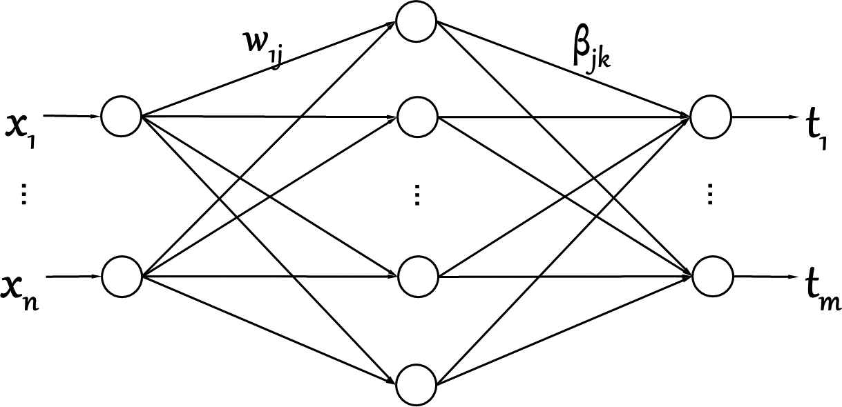
Extreme learning machine (ELM) structure.
2.2. S-ELMs
The S-ELMs divides a single large ELM network into multiple stacked small ELMs. S-ELMs can use small memory to approximate very large ELM network requirements. The main idea is to keep the size of the entire network fixed. They choose the top few significant nodes using their output weights' eigenvalues, and reduce the nodes by multiplying the corresponding eigenvectors. This can be done by performing PCA dimension reduction on the output weights calculated in each small ELM. In PCA process, the top
Step 1: Randomly generate hidden layer parameters input weight
Step 2: Use the PCA to reduce the dimension of
Step 3: Repeat the following steps until the
randomly generate
combine important nodes
hidden layer output matrix:
repeat calculate
Step 4: The output of last layer of the S-ELMs network is
3. PROPOSED STAR-ELM
3.1. Selection of Hidden Layer Parameters
One of the main features of the ELM is to randomly generate the values of hidden layer parameters, but the disadvantage is that the accuracy of the network model in the application process cannot be guaranteed, and it needs to be adjusted manually, which is a very cumbersome and time-consuming process.
For this reason, Star-ELM has improved in the parameter selection process of the hidden layer. The parameter selection does not need to be adjusted manually, which greatly improves the accuracy of the prediction model.
The main idea is to add a loop program into the traditional ELM. By customizing the number of loops
3.2. Node Sensitivity
This section describes the definition of node sensitivity in the Star-ELM, which is mainly referred to as the sensitivity to the weight value. In other words, we use quantization to calculate the effect of the output due to changes in the model parameters. That is to say, if the change of a parameter has a large impact on the output, the parameter is sensitive. On the contrary, it indicates that the parameter has little influence on the network structure. You can consider deleting it to make the network structure more streamlined. The calculation method of sensitivity is specifically described below.
There are
We can define
Without loss of generality, suppose we delete the hidden layer node
A larger
3.3. Hidden Layer Node Merge Operation
The calculation method of node sensitivity is described in detail in the previous section. In this section, the combination of nodes and layer generation between the layers is introduced for a Star-ELM. First, starting from a simple ELM network with
The nodes in the hidden layer of the network structure are merged in pairs. We chose two adjacent nodes for comparison, because the algorithm is easier to understand and implement in this way. The merge process is based on the sensitivity of the nodes, and the nodes with high sensitivity will be retained, as
In order to ensure the consistency of the number of hidden layer nodes in the second layer and the first layer, the remaining
The second hidden layer in Star-ELM formed after the combination is
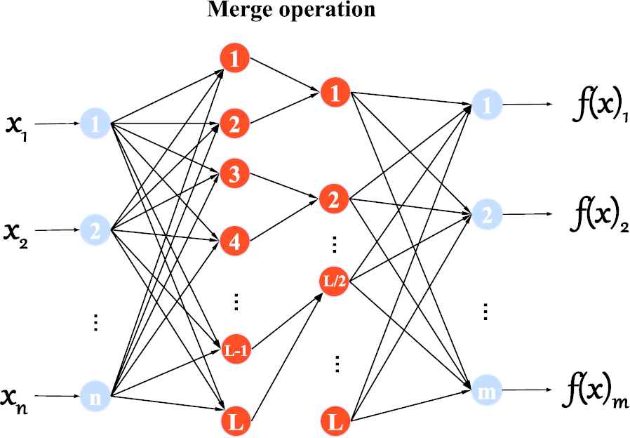
Scalable Real-Time Attributes Responsive Extreme Learning Machine (Star-ELM) structure.
After the nodes in the first hidden layer have been subjected to the calculation of the sensitivity level, the adjacent nodes are merged in pairs, and relatively important nodes were retained during the merge process, thereby discarding a part of the redundant nodes.
After obtaining nodes that can represent important information of the layer, some new nodes are randomly generated, and the two types of nodes will merge into nodes of the second hidden layer. Through the integration of important nodes in the first layer, the network structure can better adapt to the changes in different datasets. Especially when some attributes in the dataset are lost or face unbalanced datasets, the network structure has better adaptability than traditional network structures.
It is worth noting that, unlike the method of globally selecting nodes based on importance, such as S-ELMs based on PCA operation, the method proposed in this article is a local selection based on importance. When some attributes of the sample are lost, or the samples are not balanced, this method can weigh the impact of these attributes in a more balanced way, rather than discarding all unimportant nodes.
3.4. Star-ELM
According to the above improvements on the selection of hidden layer parameters, node sensitivity definition and description of hidden layer node merging, this section gives detailed steps of Star-ELM.
Given a training dataset with
The initial weights
The parameters
Calculate all
Solving the weight
Calculating the sensitivity value
Obtain the nodes' sensitivities and combine the nodes in pairs as
whereAfter the nodes are merged, a new output matrix
Solving the weight
It can be seen from the above description of the principle and steps of the Star-ELM algorithm that the hidden layer nodes in the improved algorithm can be adjusted, and the parameters involved in the operation in the first hidden layer are most suitable for the network structure. In order to prove that the algorithm has better performance than the traditional ELM, in the next section, the classic dataset is selected to verify the validity of the algorithm classification.
The algorithm for Star-ELM is summarized in Table 1.
| Algorithm 1: | Pseudo code for Star-ELM |
|---|---|
| Input: | |
| Output: | |
| 1: | Initial weights |
| 2: | Multiple runs to select best |
| 3: | Calculate |
| 4: | Combine hidden layer output matrix |
| 5: | Solving output weight matrix |
| 6: | Calculate node sensitivity |
| 7: | Merge sensitivity coefficients in pairs |
| 8: | Obtain a new output matrix |
| 9: | Randomly generate new nodes |
| 10: | Merge into |
| 11: | Calculate output value |
| Return |
Star-ELM, Scalable Real-Time Attributes Responsive Extreme Learning Machine.
Star-ELM algorithm.
4. EXPERIMENTS
4.1. Datasets
This section will check the performance of proposed Star-ELM and ELM, S-ELMs on three datasets: Modified National Institute of Standards and Technology database(MNIST), NYU Object Recognition Benchmark(NORB) and US Postal(USPS) data.
The MNIST [19] database of handwritten digits is a popular database for many researchers to do different machine learning algorithms. It consists of 60000 training samples and 10000 testing samples, each sample have 784 features. Many methods have been tested on this dataset including many other classification algorithms.
The NORB [20] dataset is for experiments in 3-D object recognition from shape. It contains 23000 training samples and 23000 testing samples with 2048 features.
The USPS [21] dataset refers to numeric data obtained from the scanning of handwritten digits from envelopes by the U.S. Postal Service. It contains 7291 training instances and 2007 testing instances with 256 features.
4.2. Experimental Environment
The simulations are carried out in the MATLAB 2016a environment running on an Intel(R) i5–3210M computer with 2.50G Hz and 4GB RAM.
4.3. Mode of Evaluation
To evaluate the performance of a classification algorithm, it is usually judged from two aspects: the time spent in the work and the accuracy of the classification accuracy. In dealing with classification problems, the most important issue of concern is the accuracy of classification. The classification ability of the model is obtained by calculating and recording the test accuracy. In this experiment, the performance of the algorithm was evaluated by the test accuracy and training time of the classification results.
In this experiment, the traditional ELM method uses 500 hidden layer nodes, S-ELMs uses two hidden layers, each hidden layer has 200 nodes. Proposed Star-ELM takes
4.4. Results
The training, test accuracy(%) and training time (
| Dataset | Algorithm | Train Accuracy (%) | Test Accuracy (%) | Time ( |
|---|---|---|---|---|
| MNIST | ELM | 85.23 | 80.12 | 3.2313 |
| S-ELMs | 86.71 | 87.77 | 4.7390 | |
| Star-ELM | 80.07 | 81.29 | 11.324 | |
| NORB | ELM | 80.39 | 78.13 | 8.1256 |
| S-ELMs | 80.01 | 79.86 | 3.0075 | |
| Star-ELM | 86.90 | 84.05 | 10.321 | |
| USPS | ELM | 89.08 | 73.14 | 2.3906 |
| S-ELMs | 94.02 | 89.88 | 5.2851 | |
| Star-ELM | 95.20 | 92.99 | 12.234 |
ELM, extreme learning machine; Star-ELM, scalable real-time attributes responsive extreme learning machine; S-ELM, stacked extreme learning machine.
Performance of different algorithms.
As shown in the Table 2, from the perspective of test accuracy, the Star-ELM algorithm has significantly higher test accuracy on the NORB and USPS datasets than the S-ELMs and ELM algorithms. Based on the MNIST dataset, the experimental results of Star-ELM have no advantage over S-ELMs, but significantly exceed the traditional ELM.
From the perspective of training time, the traditional ELM algorithm has the shortest training time and the Star-ELM algorithm has the longest time, mainly because Star-ELM cycles for 50 times to find the best weight
4.5. Scalable Attributes Experiment
Under the complete conditions of the dataset, the advantages of Star-ELM are not well reflected, and now proceed to the next experiment. The main advantage of the Star-ELM algorithm is that the network structure can be reconstructed according to the size of the dataset, and it has better adaptability to different datasets. In this experiment, by continuously reducing the attribute values of the dataset, observe the changes in the test accuracy of different algorithms.
The first is the MNIST dataset. As shown in Table 3, the initial dataset contains 784 features, and its attribute value is gradually decremented from 784 to 12. The trend of the test accuracy(%) under different algorithms is observed by the change of the number of eigenvalues, as shown in Figure 3.
| Attributes | ELM-Acc (%) | S-ELMs-Acc (%) | Star-ELM-Acc (%) |
|---|---|---|---|
| 784 | 80.12 | 87.77 | 81.29 |
| 392 | 80.00 | 80.14 | 80.00 |
| 196 | 72.10 | 80.09 | 79.02 |
| 98 | 63.04 | 80.05 | 78.11 |
| 49 | 53.72 | 72.60 | 77.00 |
| 25 | 43.42 | 60.24 | 74.74 |
| 12 | 40.10 | 54.05 | 71.33 |
ELM, extreme learning machine; Star-ELM, scalable real-time attributes responsive extreme learning machine; S-ELM, stacked extreme learning machine.
Scalable attributes on MNIST dataset test.
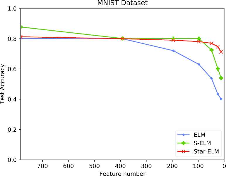
Accuracy changes for MNIST dataset test.
When the number of features in the MNIST dataset is reduced from 784 to 49, the test accuracy of the ELM is reduced from the highest precision of 80.12% to 53.72%. The accuracy of S-ELMs was reduced from 87.77% to 72.60%, while the accuracy of Star-ELM was only reduced from 81.29% to 77.00%. The decline rates of the three algorithms on the MNIST dataset are 32.95%, 17.28% and 5.28%. It can be seen that when the feature attribute is lost on the MNIST dataset, the Star-ELM can make a better adjustment of the network structure to slow down the rate of test accuracy.
Next, similar experiments were performed on the USPS dataset and the NORB dataset. As shown in Table 4 and Figure 4, when the number of features in the USPS dataset is reduced from 256 to 8, the test accuracy degradation rates of the three algorithms ELM, S-ELMs and Star-ELM are 18.56%, 51.97%, 17.75%, respectively. Among them, Star-ELM still has the lowest rate of decline on the USPS dataset, and the test accuracy is the highest when the dataset is complete. Besides, Star-ELM has also improved the classification accuracy of the dataset.
| Attributes | ELM-Acc (%) | S-ELMs-Acc (%) | Star-ELM-Acc (%) |
|---|---|---|---|
| 256 | 73.94 | 89.98 | 89.99 |
| 128 | 72.10 | 80.09 | 79.83 |
| 64 | 66.75 | 80.05 | 78.42 |
| 32 | 63.33 | 55.77 | 77.23 |
| 8 | 60.22 | 43.21 | 74.01 |
ELM, extreme learning machine; Star-ELM, scalable real-time attributes responsive extreme learning machine; S-ELM, stacked extreme learning machine.
Scalable attributes on USPS dataset test.
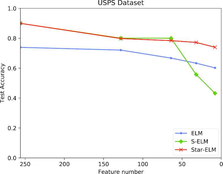
Accuracy changes for USPS dataset test.
Finally, the experiment was carried out on the NORB dataset, and the number of attribute features was gradually reduced from 2048 to 32. The performance of three different algorithms on the NORB dataset is shown in Table 5 and Figure 5.
| Attributes | ELM | S-ELMs | Star-ELM |
|---|---|---|---|
| 2048 | 73.14 | 89.98 | 85.89 |
| 1024 | 70.12 | 80.14 | 80.00 |
| 512 | 60.21 | 77.21 | 79.00 |
| 256 | 59.22 | 67.22 | 76.88 |
| 64 | 30.22 | 49.21 | 77.23 |
| 32 | 21.22 | 30.87 | 72.98 |
ELM, extreme learning machine; Star-ELM, scalable real-time attributes responsive extreme learning machine; S-ELM, stacked extreme learning machine.
Scalable attributes on NORB dataset test.
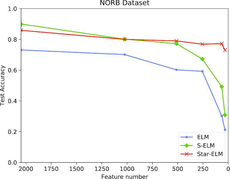
Accuracy changes for NORB dataset test.
When the number of features in the NORB data set is reduced from 2048 to 32, the test accuracy degradation rates of the three algorithms ELM, S-ELMs and Star-ELM are 70.98%, 65.69%, 15.03%. The rate of decline of ELM on the NORB dataset is still the lowest, and the accuracy of the Star-ELM algorithm is higher than that of the traditional ELM algorithm when the dataset is complete.
The main reason to get better results than ELM is that the network structure of the ELM is fixed, and it cannot be reasonably adjusted as the dataset changes. For S-ELMs, unlike the method of globally selecting nodes based on importance, used by S-ELMs, the method proposed in this article is a local selection based on importance. When some attributes of the dataset are lost, or the samples are not balanced, this method can weigh the impact of these attributes in a more balanced way, rather than discarding all unimportant nodes. Therefore, Star-ELM works better when some attributes of the dataset are missing.
5. CONCLUSIONS
This paper proposes an improved ELM algorithm Star-ELM. In order to verify that the Star-ELM can still be effectively classified during the change of the dataset. The test accuracy of different algorithms will decrease as the feature attributes are lost, but the rate of decrease is different. With the reduction of the number of features in the MNIST, USPS and NORB datasets, Star-ELM's test accuracy declines the slowest. The future work will focus on incremental network, by transferring the learning ability of Star-ELM and process the new incoming big data more effectively.
CONFLICT OF INTEREST
We declare that we have no financial and personal relationships with other people or organizations that can inappropriately influence our work.
AUTHOR CONTRIBUTIONS
Hongbo Wang, Yuejuan Yao, Xi Liu contributed to the conception of the study; Yuejuan Yao, Xi Liu performed the experiment; Hongbo Wang, Yuejuan Yao contributed significantly to analysis and manuscript preparation; Hongbo Wang, Xi Liu performed the data analyses and wrote the manuscript; Xi Liu, Xuyan Tu helped perform the analysis with constructive discussions.
ACKNOWLEDGMENTS
This work is supported by National Natural Science Foundation of China (NSFC) under Grant NO.61572074.
REFERENCES
Cite this article
TY  - JOUR
AU  - Hongbo Wang
AU  - Yuejuan Yao
AU  - Xi Liu
AU  - Xuyan Tu
PY  - 2020
DA  - 2020/08/10
TI  - Scalable Real-Time Attributes Responsive Extreme Learning Machine
JO  - International Journal of Computational Intelligence Systems
SP  - 1101
EP  - 1108
VL  - 13
IS  - 1
SN  - 1875-6883
UR  - https://doi.org/10.2991/ijcis.d.200731.001
DO  - 10.2991/ijcis.d.200731.001
ID  - Wang2020
ER  -