
Incorporating Active Learning into Machine Learning Techniques for Sensory Evaluation of Food

- DOI
- 10.2991/ijcis.d.200525.001How to use a DOI?
- Keywords
- Sensory evaluation of food; Active learning; Machine learning
- Abstract
The sensory evaluation of food quality using a machine learning approach provides a means of measuring the quality of food products. Thus, this type of evaluation may assist in improving the composition of foods and encouraging the development of new food products. However, human intervention has been often required in order to obtain labeled data for training machine learning models used in the evaluation process, which is time-consuming and costly. This paper aims at incorporating active learning into machine learning techniques to overcome this obstacle for sensory evaluation task. In particular, three algorithms are developed for sensory evaluation of wine quality. The first algorithm called Uncertainty Model (UCM) employs an uncertainty sampling approach, while the second algorithm called Combined Model (CBM) combines support vector machine with Density-Based Spatial Clustering of Applications with Noise (DBSCAN) algorithm, and both of which are aimed at selecting the most informative samples from a large dataset for labeling during the training process so as to enhance the performance of the classification models. The third algorithm called Noisy Model (NSM) is then proposed to deal with the noisy labels during the learning process. The empirical results showed that these algorithms can achieve higher accuracies in this classification task. Furthermore, they can be applied to optimize food ingredients and the consumer acceptance in real markets.
- Copyright
- © 2020 The Authors. Published by Atlantis Press SARL.
- Open Access
- This is an open access article distributed under the CC BY-NC 4.0 license (http://creativecommons.org/licenses/by-nc/4.0/).
1. INTRODUCTION
In food industry, the evaluation of food quality plays an important role in food manufacturing and food-consumption market. In food manufacturing, it enables improvement in food ingredients employed by suggesting appropriate changes in the physico-chemical properties of food. In food-consumption market, it can successfully suggest foods offered to consumers meeting or even exceeding their expectations. In fact, food quality not only benefits us by defining a set of food attributes that meet consumer expectations, but also allowing us to determine food product requirements. According to [1], several attributes play an important role in consumer acceptance of foods including nutritional value and the sensory attribute. Nutritional value is the basic attribute of food that enables it to nourish us, while sensory attribute is a critical property in several dimensions of food quality that forms a system for measuring the quality of a food product. In addition, many factors can affect consumer's consumption for food products, including trademark image, price, and rival position. However, the most important factor is consistently supplying sensory characteristics that consumers can perceive in assessing the quality of food products. Consequently, food quality can be seen as the sum of several partial qualities, such as quality of raw materials used in the food's preparation, production technology, and sensory quality [2]:
Human senses can be easily used to analyze and evaluate the sensory quality that constitutes such characteristics as color, shape, size, smell, taste, and structure [3]. However, this kind of evaluation is typically difficult and time-consuming to collect and often uncertain as well. In addition, there are two phases in this process. First, a sensory analysis method is used to assess the food's sensory attributes, and then experts use these results in a formalized and structured method to evaluate specific food products. In order to ensure acceptable product quality, the sensory evaluation should be performed throughout the food manufacturing process from the selection of raw materials, to the final product meets the desired quality. Besides that, to control the quality of food products, other methods, such as chemical, physical, and microbiological tests must be performed as well [2].
So far, many data mining approaches such as data synthesis, clustering, and classification [4–8] have been applied to automatically assess sensory quality. For instance, Cortez et al. [9] investigated the use of support vector machine (SVM), multiple regression (MR), and neural network (NN) methods to predict the quality of different kinds of wine from their physico-chemical characteristics. The results showed that SVM performed well in predicting the wine preferences from class 3 to class 8, with an accuracy higher than 86% with the tolerance value of 1.0. However, one disadvantage of this approach is the need of labeled data, which requires an extreme effort to produce. However, in comparison with traditional techniques, data mining methods are more robust, faster, and cheaper. In spite of these advantages, human perceptions are quite complicated and therefore cannot completely be replaced by machines. Thus, combining human efforts and computers for evaluating food products is an interesting task.
In this research, we introduce a combination approach involving humans and machines to address the sensory analysis task. Our study involves an analysis of wine quality as in [9] and propose three contributions. First, we introduce two algorithms for sensory evaluation of food that employ active learning. The first algorithm is used to investigate the most uncertainty sampling, while the second algorithm combines SVM classification algorithm with Density-Based Spatial Clustering of Applications with Noise (DBSCAN) clustering algorithm to select the most informative samples. These methods initially choose a small set of available training data provided by human analyzers. Then, it iteratively classifies the wines and chooses the one that was judged as the most informative. An expert is then asked to label the sample, which is used as an additional resource for the algorithms to improve the classification accuracy. By this way, these two proposed algorithms are able to reduce the number of samples that need to be labeled. Next, we propose the third algorithm which deals with noisy labels. The third contribution of our research is the empirical experiments that were conducted on a real-world dataset to evaluate the performance of the proposed algorithms. The paper is organized as follows: Section 2 briefly recalls some related work and Section 3 provides preliminaries on active learning and several data mining techniques used for sensory evaluation of food, including sequential minimal optimization (SMO), decision tree (DT), random forests (RFs), and NN. Section 4 presents the proposed algorithms and Section 5 describes the experimental results. Finally, Section 6 draws the conclusion and discusses the future research.
2. RELATED WORK
In recent decades, the food and beverage industry has employed a broadly developed and designed system to automatically evaluate product quality. This task has played an important role in improving food quality through the choice of ingredients and the marketing campaign. Traditional methods such as principal component analysis (PCA) [10] have been used to analyze food's sensory data, that is supported by experts. This method can effectively solve for some specific tasks, but may lead to the loss of important information. To overcome this limitation, several methods have been proposed, including RFs [11], NN [4,12], fuzzy logic [5,7,13], and SVMs [8,9,14], to resolve the uncertainty problem in sensory evaluation.
Nowadays, many researchers have applied different approaches that involve data mining to identify food products' physical and chemical ingredients, which are the key features to evaluate the food's sensory quality. For example, Debska et al. [4] employed an artificial neural network (ANN) in a learning model to classify Poland's beer quality based on its chemical characteristics. Their results demonstrated the effectiveness of using an ANN in classifying the quality of beer products. Cortez et al. [9] investigated several data mining techniques including SVM, MR, and NN to predict the quality of white and red “Vinho Verde” wine of Portugal. The obtained result indicated that SVM outperformed MR and NN, and it can be used as an effective model to support experts in wine quality classification.
In order to help companies in making marketing campaign, Ghasemi-Varnamkhasti et al. [15] employed a NN model to evaluate the sensory characteristics of commercial non-alcoholic beer brands and found that the radial basis function provided a successful grading rate of about 97%. Thus, this approach can be used as a decision support model for electronic noses and electronic blades in beer quality control. Sensory evaluation plays a very important role in controlling quality of beer. Dong et al. [14] studied some nonlinear models including partial least squares, genetic algorithm back-propagation NN, and SVM to define the relationship between a flavor compound and sensory evaluation of beer. The results showed that the SVM model performed better than other models, with 94% accuracy. Thus, SVM is a powerful method that has great potential for evaluating beer quality.
To sum up, data mining techniques have some advantages in sensory quality assessment of food products. It is also demonstrated that physico-chemical properties of food products can be used to classify the sensory quality of food products by a learning model. Therefore, data mining techniques can be used to assist food organizations in enhancing the quality of food products. At the same time, however, they often require high cost and time consuming in the labeling task. For example, a study on the sensory quality of lamb from November 2002 to November 2003 used 81 samples for each animal, and it costed 6 Euros per kilogram, and thus the entire experiment involved a significant cost [8]. Therefore, a less costly and time-consuming system is needed. This motivated us proposing to incorporate active learning into the learning framework as developed in this paper.
3. PRELIMINARIES
In this section, we recall basic of active learning and then discuss several classifier techniques, such as SMO, DT, RFs, and NN in Section 3.2.
3.1. Active Learning
Instead of passively using all training samples provided to study, active learning algorithms automatically choose the ones they need in order to learn to enhance their performance [16]. Figure 1 illustrates a general scenario for active learning methods.
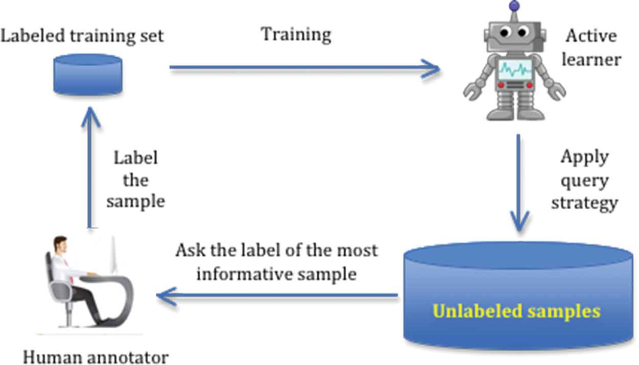
The active learning process.
Typically, active learning algorithms start with a small labeled training sample employed to teach the classifier. Then, an active learner of the algorithm will examine the results and choose the most informative samples from a set of unlabeled samples. These selected samples will be given to human annotators to manually label according to their judgment. Labeled instances will then be included in the training set to initialize a new training phase. The whole process is then repeated until the user query budget is exceeded. This scheme significantly enhances classification accuracy as well as reduce human annotation efforts. Thus, it has been widely used in many fields such as in [16–18].
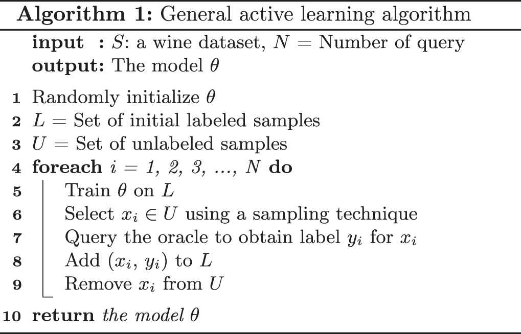
The workflow of a general active learning algorithm applied in a wine-related context is described in the Algorithm 1 as follows: A wine dataset
3.2. The Classifiers
The sampling strategy of active learning requires classifiers to predict unlabeled data. Our proposed algorithms use SMO, DT, RF, and NN for this purpose.
Sequential minimal optimization: The SMO algorithm was introduced by J. Platt [19]. It used to train the SVM model by quickly solving a very large quadratic programming (QP) optimization problem by dividing it into a series of smaller QP problems. The SMO's advantages are that large matrices do not need to be stored and that each QP sub-problem can be initialized with the results of solving the previous sub-problems. The key idea of SMO is to make use of selection to deal with optimization processes. At each step, the SMO chooses two Lagrange multipliers to optimize simultaneously. Then, after finding optimal values for these multipliers, it updates the SVM to obtain new optimal values. Thus, the SMO performs two primary tasks: finding an optimal solution for two Lagrange multipliers and a heuristic method for selection of these two multipliers. The SMO algorithm has two following advantages. First, it eliminates the high computational cost and memory usage needed to solve the large QP optimization problems associated with SVM, making it highly suitable for handling large datasets such as those used to train machine learning algorithms. Second, the SMO speeds up solution of a linear SVM and reduces the amount of data needed to be stored to only a single weighting vector. Therefore, in this paper we employed the SMO algorithm to minimize the running time of the proposed algorithms' training process.
Decision Tree: The DT [20] is a structured hierarchy used for classification and prediction. The topmost node in the DT is the root node, and the children nodes below it in the tree are internal nodes and leaf nodes. Each internal node represents an attribute, while its branches and leaf nodes represent possible values of the attribute and decision classes, respectively. The algorithm is initialized with the root node and proceeded along the branches of the tree to leaf nodes. In data mining, a DT can be used to classify data into one of two or more categories, and the DT can be transformed into decision rules. Several widely DT algorithms are used as ID3 and C4.5. Figure 2 below shows the DT of the first fifteen samples of the white wine dataset (Section 5.1).
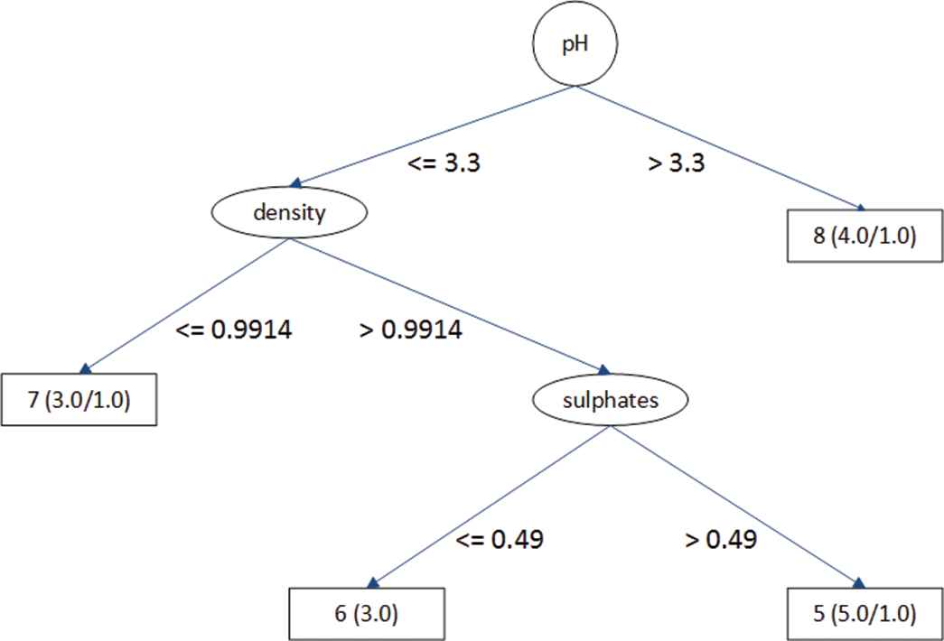
The decision tree (DT) of the first fifteen samples of the white wine dataset.
Random Forest: Firstly proposed by Leo Breiman [21], the RF algorithm is a classification and regression method based on the combination of the predicted results of a large number of DTs. In the RF model, each tree predictor is constructed randomly from a smaller dataset, which is divided from the original dataset. Child nodes are developed from a parent node based on the information in the subspace, which selects informative attributes from the original attribute space. Ultimately, the RF constructs tree predictors from a subset of randomly selected attributes and then synthesizes the trees' predicted results to produce a final prediction. To minimize the correlation between these tree predictors, the subspace attributes are selected randomly. Therefore, combining the results of a large number of independent tree predictors having low deviation and high variance will help RF achieve both low deviation and low variance. The accuracy of RF model depends on the predictive quality of the tree predictors and the degree of correlation between them.
Neural network: NN [20] is a machine learning model that mimics the operation of the human nervous system. Basically, the NN consists of processing units that communicate signals to other units through weighted links. NN learning algorithms typically use a gradient descent method to adjust network parameters to fit a training set. One of NN's primary advantages is that it can work well with unconstructed data with a high accuracy. One significant limitation of NN is that its training process requires a large number of labeled samples. NNs have been widely applied in many fields including speech recognition, image processing, prediction, forecasting, analysis of visual data, and learning-based robot control strategies. Typical NN models incorporate such machine learning techniques as feedforward NNs, multi-layer perceptrons, radial basis function networks, Kohonen self-organizing maps, and recurrent neural networks (RNNs).
4. THE PROPOSED ALGORITHMS
In this section, we propose three algorithms for the wine classification problem. The first algorithm denoted by Uncertainty Model (UCM) uses an uncertainty sampling approach (Algorithm 2), while the second algorithm denoted by Combined Model (CBM) is used for sampling selection (Algorithm 3). The third algorithm called Noisy Model (NSM) is used for dealing with noisy samples (Algorithm 4).
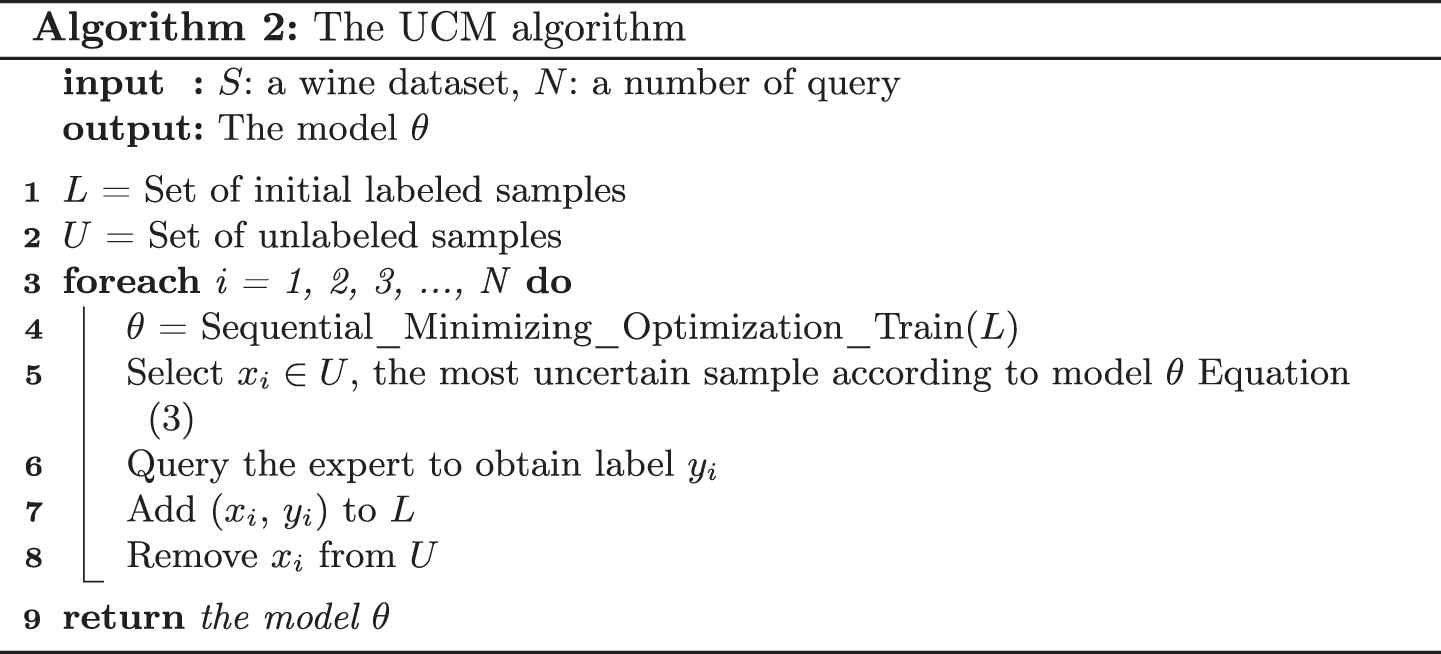
The UCM algorithm: The UCM algorithm employs SMO as its primary classification technique and the pool-based uncertainty sampling algorithm for active query selection. Algorithm 2 provides the pseudocode of this technique.
In this research, dataset
The entropy computation (Equation 1) [22] is used to define the most uncertain sample, i.e. the sample with the highest entropy.
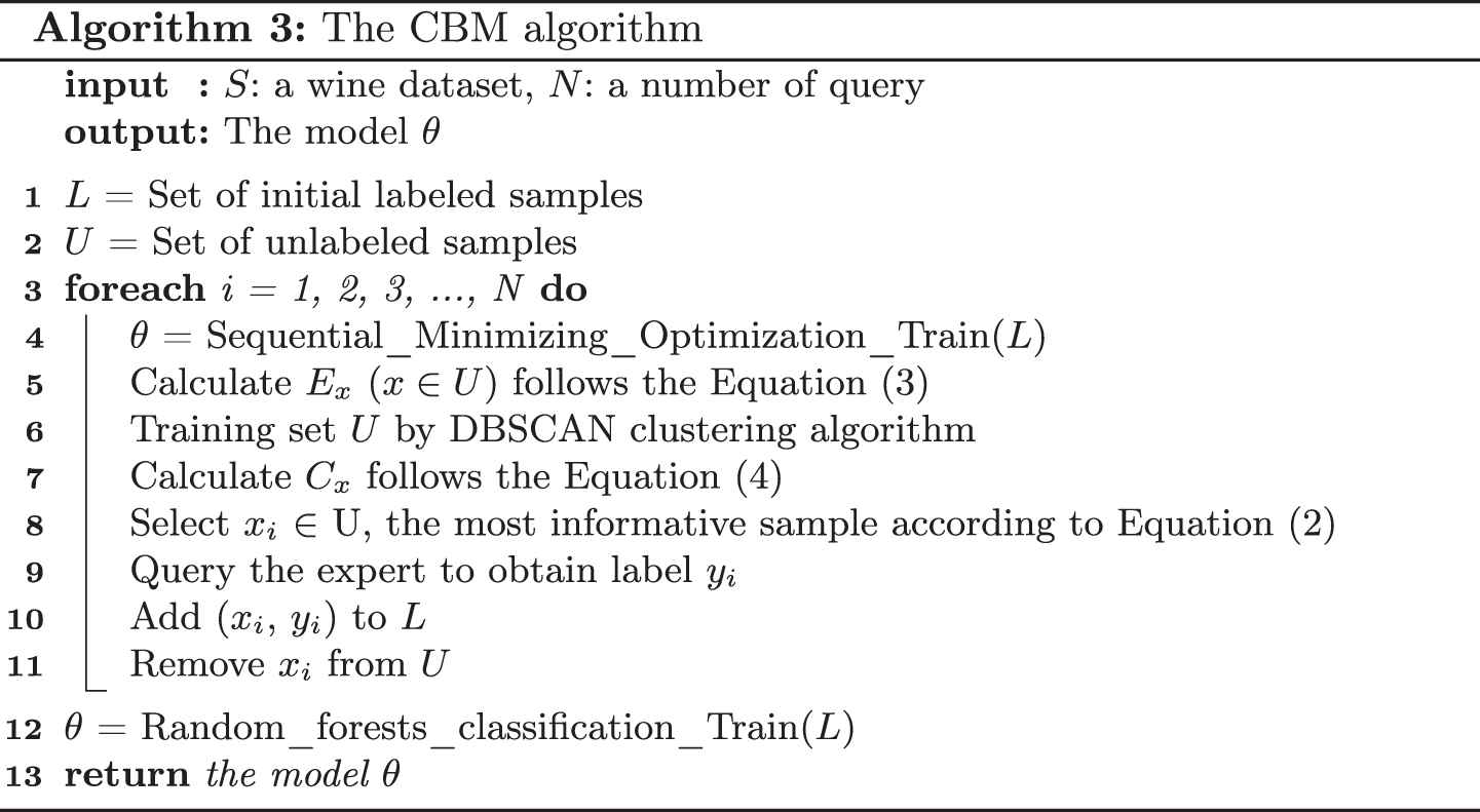
The CBM algorithm: The CBM algorithm employs SVM as its primary classification technique and the DBSCAN algorithm for clustering. The combination of these two techniques is used to choose the most informative samples for updating the labeled dataset
At each stage of the CBM algorithm, the model applies the SMO technique to train the classification model
Note that, here we propose a new way to calculate the most informative sample as follows:
The information density computation
The NSM algorithm: The third proposed algorithm NSM is developed for dealing with noisy labels which would be wrongly labeled by active learning strategies. It combines three classification techniques including SVM, DT, and NN as shown as in Algorithm 4.
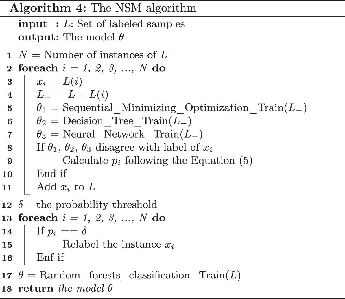
As the expert might be potentially wrong in labeling data and such newly added samples could cause noise in the resulting labeled dataset
5. EMPIRICAL RESULTS
This section describes an empirical experiment conducted on a real-world dataset for evaluating the performance of the UCM, CBM, and NSM algorithms. Specifically, we evaluated the performance of these three algorithms with respect to classification accuracy using the Wine dataset [23].
5.1. Wine Dataset
Cortez et al. [9] contributed a dataset collected from May, 2004 to February, 2007 for the sensory quality of wines grown in the Minho region of Portugal. This dataset was tested at official certification entity (CVRVV). The dataset of red wine contains 1,559 samples, while the dataset of white wine contains 4,898 samples. These datasets can be found in the UCI archives [23].
For both datasets, the input variables are the physiochemical characteristics that include fixed acidity, volatile acidity, citric acid, residual sugar, chlorides, free sulfur dioxide, total sulfur dioxide, density, pH, sulphates, and alcohol. The output results are the wine's quality.
Tables 1 and 2 provide the descriptive statistics of the physico-chemical components of the red and white wine datasets, respectively. At least three sensory assessors (using blind tastes) were required to evaluate each sample in the dataset, with each wine's final score is calculated by taking the mean of these expert evaluations. The score of sensory quality ranged from 0 (very bad) to 10 (excellent).
| Physicochemical | Min | Max | Mean | StdDev |
|---|---|---|---|---|
| Fixed acidity | 4.600 | 15.900 | 8.320 | 1.741 |
| Volatile acidity | 0.120 | 1.580 | 0.528 | 0.179 |
| Citric acid | 0.000 | 1.000 | 0.271 | 0.195 |
| Residual sugar | 0.900 | 15.500 | 2.539 | 1.410 |
| Chlorides | 0.012 | 0.611 | 0.087 | 0.047 |
| Free sulfur dioxide | 1.000 | 72.000 | 15.875 | 10.460 |
| Total sulfur dioxide | 6.000 | 289.000 | 46.468 | 32.895 |
| Density | 0.990 | 1.004 | 0.997 | 0.002 |
| pH | 2.740 | 4.010 | 3.311 | 0.154 |
| Sulphates | 0.330 | 2.000 | 0.658 | 0.170 |
| Alcohol | 8.400 | 14.900 | 10.423 | 1.066 |
The red wine data statistics.
| Physicochemical | Min | Max | Mean | StdDev |
|---|---|---|---|---|
| Fixed acidity | 3.800 | 14.200 | 6.855 | 0.844 |
| Volatile acidity | 0.080 | 1.100 | 0.278 | 0.101 |
| Citric acid | 0.000 | 1.660 | 0.334 | 0.121 |
| Residual sugar | 0.600 | 65.800 | 6.391 | 5.072 |
| Chlorides | 0.009 | 0.346 | 0.046 | 0.022 |
| Free sulfur dioxide | 2.000 | 289.000 | 35.308 | 17.007 |
| Total sulfur dioxide | 9.000 | 440.000 | 138.361 | 42.498 |
| Density | 0.987 | 1.039 | 0.994 | 0.003 |
| pH | 2.720 | 3.820 | 3.188 | 0.151 |
| Sulphates | 0.220 | 1.080 | 0.490 | 0.114 |
| Alcohol | 8.000 | 14.200 | 10.514 | 1.231 |
The white wine data statistics.
Figure 3 illustrates the distribution of the red wines and white wines over eleven levels of sensory preferences. Both figures display a typical unimodal normal shaped distribution.
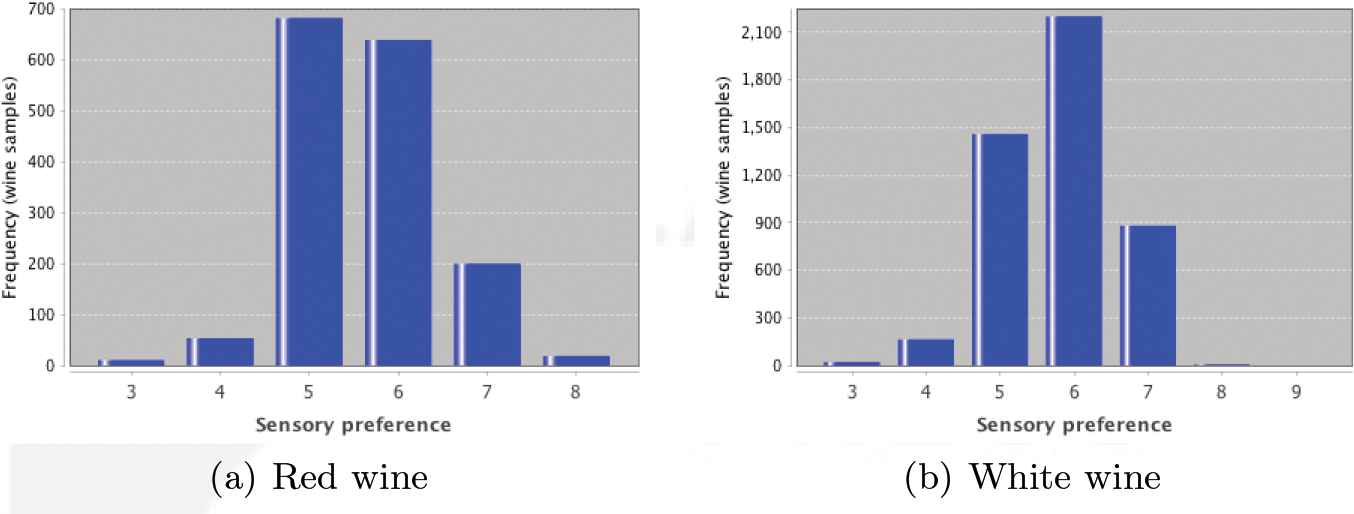
The histograms for the red and white sensory preferences.
5.2. Results
The experiments designed to evaluate the performance of the two proposed algorithms were carried out on a computer with a 1.7 GHz Intel core i7, 8 GB of RAM, running on MacOS High Sierra operation using Java programming. The number of initial labeled instances was set at 10, and the number of queries is 100. In addition, we employed a 10-fold cross validation for evaluating the models.
For the sake of comparison, the general active learning algorithm employing random sampling (RDM) is also used in the experiment and its results are included. As Figure 4 shows, for both wine datasets, the classification accuracy of the CBM algorithm completely outperformed both UCM and RDM. For the red wine dataset, the highest classification accuracy obtained by the CBM algorithm, the UCM algorithm, and the RDM were 74%, 71%, and 47%, respectively. While for the white wine dataset, the highest accuracy of the CBM, UCM, and RDM algorithms are 71%, 57%, and 41%, respectively. Also, the CBM algorithm showed a gradually increasing trend of the classification accuracy along the number of queries.
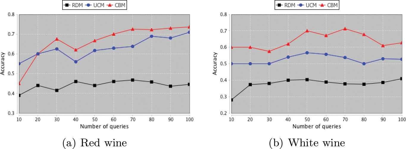
The classification accuracy of Combined Model (CBM), Uncertainty Model (UCM), and random sampling (RDM) algorithms per wine type.
In order to deepen the analysis of the sensory perception of wine, Cortez et al. [9] employed a predefined acceptable threshold
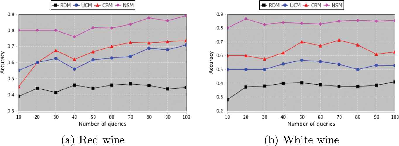
The classification accuracy of all four models per wine type.
6. CONCLUSIONS
The results of our empirical experiments confirmed that a data mining approach can successfully obtain comparative results on classification accuracy for classifying wine preference based on the sensory attributes. Moreover, combining classification algorithm and clustering algorithm with an active learning technique can be able to enhance the accuracy of the learning model. One advantage of this approach is to assist human analysis by automatically evaluating the sensory evaluation of food products. This approach could be used to reduce the cost of labeling data process, which involves experts in the classification task. It also helps models boost the classification accuracy without having any hand-crafting knowledge or numerous number of labeled dataset, which is the primary drawback of machine learning technique. It can reduce the costly money of collecting and labeling such data, in order to minimize the time-consuming process.
On both wine datasets, the UCM, CBM, and NSM algorithms combined with an intelligent strategy of sampling selection had outperformed a random sampling approach. In particular, for the red and white wine datasets, the NSM algorithm achieved maximum accuracy of around 89% and 87% respectively, with the tolerance
CONFLICT OF INTEREST
The authors declare no conflicts of interest for this article.
AUTHORS' CONTRIBUTIONS
N.-V.L., T.Y. and V.-N.H. conceived of the presented idea. N.-V.L. developed the proposed model and performed the experiments. R.T. and T. Y. supported N.-V.L. in performing the analysis and interpretation of results. All authors discussed the results, provided critical feedback, and helped shape the research, analysis, and manuscript. N.-V.L. and V.-N.H. wrote the manuscript in consultation with R.T. and T.Y. V.-N.H. submitted the manuscript for publication and communicated with the journal editor.
ACKNOWLEDGMENTS
The authors are very grateful to the anonymous reviewers and Associate Editor for their insightful and constructive comments that have helped to significantly improve the presentation of this paper.
REFERENCES
Cite this article
TY  - JOUR
AU  - Nhat-Vinh Lu
AU  - Roengchai Tansuchat
AU  - Takaya Yuizono
AU  - Van-Nam Huynh
PY  - 2020
DA  - 2020/06/12
TI  - Incorporating Active Learning into Machine Learning Techniques for Sensory Evaluation of Food
JO  - International Journal of Computational Intelligence Systems
SP  - 655
EP  - 662
VL  - 13
IS  - 1
SN  - 1875-6883
UR  - https://doi.org/10.2991/ijcis.d.200525.001
DO  - 10.2991/ijcis.d.200525.001
ID  - Lu2020
ER  -