
An Integrated Decision Framework for Group Decision-Making with Double Hierarchy Hesitant Fuzzy Linguistic Information and Unknown Weights
 , Samarjit Kar3
- DOI
- 10.2991/ijcis.d.200527.002How to use a DOI?
- Keywords
- Bayesian approximation; Borda method; Double hierarchy hesitant fuzzy linguistic term set; Evidence theory; Group decision-making; Maclaurin symmetric mean
- Abstract
As an attractive generalization to hesitant fuzzy linguistic term set, double hierarchy hesitant fuzzy linguistic term set (DHHFLTS) is used to represent complex linguistic expressions by providing rich and flexible context. Previous studies on DHHFLTS show that aggregation of preference information does not consider the interrelationship among attributes. Motivated by this challenge, in this paper, we extend the generalized Maclaurin symmetric mean (GMSM) operator to DHHFLTS. The GMSM operator is highly generalized and captures the interrelationship among attributes effectively. The attributes' weight values are determined by using statistical variance method under DHHFLTS context. The decision makers' weights are calculated by using newly proposed evidence theory-based Bayesian approximation method with double hierarchy preference information. A new extension to the Borda method is provided under DHHFLTS context for prioritizing objects. Also, the applicability of the proposed method is demonstrated by using a green supplier selection problem for a sports company. Finally, the superiorities and limitations of the proposed method are discussed in comparison with similar methods.
- Copyright
- © 2020 The Authors. Published by Atlantis Press SARL.
- Open Access
- This is an open access article distributed under the CC BY-NC 4.0 license (http://creativecommons.org/licenses/by-nc/4.0/).
1. INTRODUCTION
Linguistic decision-making [1] is a popular and powerful concept that provides a rich and flexible environment for decision makers (DMs) to elicitate their preference over a specific alternative. Herrera et al. [2] framed the genesis of linguistic term set (LTS) and applied the same for multi-attribute decision-making (MADM). The main limitation of LTS is that it can represent complex linguistic expressions effectively. To address the limitation, Rodriguez et al. [3] proposed a hesitant fuzzy linguistic term set (HFLTS) which combines the strength of both hesitant fuzzy set (HFS) [4] and LTS. Attracted by HFLTS, many scholars extended aggregation operators [5–8], distance measure/operational laws [9] and ranking methods [10,11] to HFLTS context. Recently, Liao et al. [12] conducted a survey on HFLTS and presented its key role in MADM. Later, Rodriguez et al. [13] analyzed different linguistic models and identified that these models (including HFLTS) cannot be used for representing complex linguistic expression such as “not so good” and “somewhat satisfied.” Intuitively, to circumvent this issue, possible linguistic combinations must be enhanced for better representing complex expressions like “so bad” and “somewhat bad.”
Inspired by the idea, Gou et al. [14] proposed the double hierarchy hesitant fuzzy linguistic term set (DHHFLTS), which provides two hierarchies that are independent of each other and the secondary hierarchy is the concrete supplement of the primary hierarchy. They claimed that DHHFLTS can handle complex linguistic expressions effectively, but probabilistic linguistic term set (PLTS) can associate probability of occurrence for each term in MADM. Since the focus of this paper is pertaining to DHHFLTS, we request readers to refer [15] for clarity on the PLTS concept. The DHHFLTS provides a rich and flexible environment for preference elicitation by offering a linguistic combination of
Motivated by these train of thoughts, in this paper, we adopt an DHHFLTS as the preference style. Further, Maclaurin symmetric mean (MSM) operator [24] is a mean-based aggregation operator that considers both the weights of DMs and the risk appetite values of the DMs. It has the ability to effectively capture the interrelationship between among attributes. Attracted by the power of MSM many researchers used the operator for aggregating preferences of various styles. A comprehensive literature analysis on the extensions of MSM operators to different preference models are given below.
Liu et al. [25] proposed interval-valued linguistic intuitionistic fuzzy MSM operator for site selection with weights of attributes and DMs obtained directly. Peng [26] extended the MSM operator to single-valued neutrosophic fuzzy set and performed teacher selection by directly considering weights of attributes and DMs. Feng et al. [27] proposed 2-tuple linguistic dependent fuzzy-based geo-MSM operator for company selection with direct elicitation of weight values. Wang et al. [28] extended the MSM operator to interval-valued 2-tuple pythagorean fuzzy set and utilized the same for green supplier evaluation with weight information obtained directly. Bai et al. [29] proposed partitioned MSM operator under q-rung orthopair fuzzy context for investor selection problem with DMs' weights calculated using power method. Further, Yu et al. [30] presented a new extension to MSM operator under HFLTS and used the same for country selection to expand market. Wang et al. [31] developed a neutrosophic linguistic MSM operator for investor selection with weights obtained directly for evaluation. Also, Liu and Gao [32] proposed HFLTS-based generalized MSM operator with direct weight values for third-party logistic service provider selection. Wang et al. [33] proposed MSM operator under simplified neutrosophic linguistic context for hotel evaluation with weight information obtained directly for evaluation.
From the analysis made above, we can understand that the DHHFLTS has just started and there are attractive chances for exploration in the field of MADM. Moreover, MSM is a powerful operator for aggregating preferences and is widely used in different preference styles. Some challenges that can be encountered from the literature of DHHFLTS and MSM are
Weights of DMs are directly provided as input in the process of aggregation of preferences by using MSM operator which causes inaccuracies in the decision-making process. This is an interesting challenge to be addressed.
Calculation of attributes' weights by properly reflecting the DMs' hesitation in preference elicitation is also an interesting challenge to be focused under the context of DHHFLTS.
Aggregation of DHHFLTS-based preference information is also done without properly capturing the interrelationship among attributes. This is also an open challenge to be addressed.
Sensible and simple prioritization of objects under DHHFLTS context with less information loss is an important challenge to be focused.
To alleviate these challenges, we gain motivation and provide some contributions as follows:
Evidence theory is integrated with Bayesian approximation for sensibly determining the weights of DMs. Also, statistical variance (SV) method is extended to DHHFLTS context for systematic calculation of attributes weights. Hesitation in the preference information is properly captured by these methods with no apriori weight information.
Generalized Maclaurin symmetric mean (GMSM) operator is extended to DHHFLTS context for properly capturing the interrelationship among attributes.
Borda method [34] is extended under DHHFLTS context for sensible prioritization of objects with less information loss.
Finally, a numerical example of green supplier selection for a sports company is presented to validate the applicability of the proposed method. Further, a discussion is made on the superiorities and limitations of the proposed method by comparison with other methods.
The rest of the paper is organized as follows: In Section 2, the basic concept of LTS, HFLTS, and DHHFLTS are discussed. In Section 3, the core contribution of the research is provided, which includes calculation of attributes' weight values, calculation of DMs' weight values, aggregation of preferences and prioritization of objects. Section 4 presents the results and discussion which demonstrates a numerical example of green supplier selection for a sports company and conducts a comparative analysis of the proposed method with other methods. Finally, Section 5 provides the conclusion and future direction for research. Readers can refer to the Appendix section for the meaning of the notations used in this manuscript.
2. PRELIMINARIES
Let us discuss some basics of LTS, HFLTS, and DHHFLTS.
Definition 1.
[2] Consider an LTS
If
Negation of
Definition 2.
[3] Let
Here,
Definition 3.
[14] Let
For convenience, we call
Definition 4.
[14] Let
Note 1: Equations (3–5) denote addition, multiplication, scalar multiplication, and power operations, respectively.
3. PROPOSED DECISION FRAMEWORK
This section provides the core contribution for rational decision-making with DHHFLTS information. Motivated by the challenges identified from the literature analysis (refer Section 1), some research contributions are presented. Problem statement is initially framed, followed by methods for systematic calculation of DMs' and attributes' weights are presented with unknown weight information. Then, GMSM operator is extended to DHHFLTS for sensible aggregation of preferences and finally, Borda method is utilized for prioritization of alternatives with DHHFLEs.
3.1. Group Decision-Making Problem Under Uncertainty
Before discussing the core contribution of the research work in detail, let us understand the problem of group decision-making under uncertainty. Initially
3.2. Evidence Theory-Bayesian Approximation Method—DMs' Weight Calculation
In this section, we propose a systematic procedure for calculating DMs' weights. Generally, the DMs' weight values are directly provided which causes inaccuracies in the decision-making process [35]. To circumvent the issue, scholars proposed methods for calculating DMs' weight values. Zhang et al. [36] and Liu et al. [37] proposed MAGDM methods under heterogeneous context by considering individual concerns, satisfaction, and self-confidence. Recently, Koksalmis and Kabak [38] made a deep investigation on different state-of-the-art methods for deriving DMs' weight values and inferred that (i) DMs' weight values reflect their importance and reliability in the decision-making process; (ii) moreover, direct elicitation of weight values causes inaccuracies and affects rationality in decision-making; (iii) further, fuzzy-based MADM popularly use weight calculation methods for DMs and adopt static type of weighting; and (iv) finally, there is a need for DMs' weight calculation method in MADM for making rational decisions.
Motivated by these inferences, in this paper, we make an effort to calculate DMs' weight values by extending evidence theory-based Bayesian approximation method under DHHFLTS context. Gupta et al. [39] integrated the idea of evidence theory and Bayesian approximation for calculating the weights of DMs in intuitionistic fuzzy context. Some attractive advantages of the method are (i) evidence theory, also called Dempster-Shafer theory (DST) is a powerful concept for handling uncertainty in the preference information; (ii) Bayesian approximation mitigates the limitation of DST by distributing probabilities over the assertions rather than assigning them to the power set of assertions [40].
Motivated by the superiority of evidence theory-based Bayesian approximation method, in this paper, we extend the same to DHHFLTS. Let
Step 1: Let
Step 2: Weighted attribute evidence body is calculated by using Eqs. (6) and (7).
We follow the same step for all instances of secondary hierarchy.
Step 3: Bayesian approximation
Step 4: Combination rule is applied attribute-wise to fuse the composite evidence of each object over every DM by using Eq. (9).
We apply the step for all instances of primary hierarchy.
Step 5: The distance and similarity matrices are calculated using Eqs. (10) and (11) respectively and the order of the matrices are given by
From Eqs. (10) and (11) we obtain two matrices of order
Step 6: Similarity matrices are calculated for both the primary hierarchy and secondary hierarchy over every instance. The order of both the matrices are
Step 7: Support and creditability measure are calculated for each DM by using Eqs. (12) and (13) respectively.
From Eq. (13) we can clearly understand that the DM with highest creditability value is considered more important or reliable for the decision-making process and so on.
Initially, the subscript of the primary and secondary hierarchies are assigned as evidences from each decision matrix. Attributes' weights calculated from Section 3.3 are used to determine the weighted evidences for each matrix. Bayesian approximation values are calculated for the evidences and they are aggregated attribute wise. Similarity between each DM is determined by using Eq. (11). Finally, the credibility of each DM is determined by using the support value and this determines the weight of the DM in a systematic manner.
3.3. SV Method—Attributes' Weight Calculation
In this section, we put forward a systematic procedure for determining the weights of the attributes under DHHFLTS context. Previously, scholars adopted methods like AHP (analytical hierarchy process) [41], entropy measures [42,43], and optimization models [44] for weight calculation. The former two methods are used, when the weight information is completely unknown and the latter method is used, when the information is partially known. To the best of our knowledge, systematic attribute weight calculation under DHHFLTS context is lacking and in this paper, we overcome the issue by extending the SV method under DHHFLTS context. The SV method is used when the information is completely unknown. Liu et al. [45] claimed that (i) SV method is simple and straightforward; (ii) unlike other statistical methods, the SV method considers all data points before determining the distribution. Moreover, Kao [46] proved that the SV method is very powerful in reflecting the hesitation and uncertainty in preference information.
Motivated by these trains of thought, in this paper, we extend the SV method to DHHFLTS context. The systematic procedure is given below:
Step 1: Form an evaluation matrix of order
Step 2: Transform the DHHFLEs into single-valued elements by using Eq. (14).
Step 3: Calculate the mean for each attribute by using the matrix from step 2 and determine the variance for each attribute by using Eq. (15).
Step 4: From step 3, we get a variance vector of order
A new matrix of order
3.4. GMSM Operator—Preference Aggregation
This section presents a new extension to GMSM operator under DHHFLTS context. Previous aggregation operators on DHHFLTS context [14] do not properly capture the interrelationship between attributes and this causes unreasonable aggregation of preferences. GMSM operator [24] is a generalized aggregation operator that can easily derive other operators as special cases. The operator also has the ability to capture interrelationship among attributes which provides rational aggregation of preference information.
Motivated by the superiority of GMSM operator, in this paper, we extend the idea of GMSM to DHHFLTS context. The operator is defined below.
Definition 5.
The aggregation of DHHFLEs using DHHFGMSM (double hierarchy hesitant fuzzy GMSM) operator is a mapping
Here, DMs' weight values are obtained from Section 3.2. It must be noted that
Theorem 1.
The proposed DHHFGMSM operator is commutative, bounded, monotonic, and idempotent.
Commutativity If
Proof:
Since
Idempotent If
Proof:
From Eq. (17), we get
By expanding the terms, we get,
Since
Monotonicity If
Proof:
To prove monotonicity property, we must define score and deviation of DHHFLEs.
Let
Bounded If
Proof:
From monotonicity and idempotency properties, we have
Theorem 2.
The aggregation of DHHFLEs by using DHHFGMSM operator produces a DHHFLE.
Proof:
The idea to prove the theorem is to show that the aggregated value is also within the cardinality. We need to show that the subscript of the aggregated primary hierarchy is within the set
Hence,
3.5. Extending the Borda Method to DHHFLTS Context
In this section, we extend the Borda method to DHHFLTS context. Borda method is an attractive method for aggregation of preferences. The method is flexible and provides a rational decision by selecting the broadly-acceptable alternative. Garcia et al. [47] presented two variants of Borda viz., narrow and broad Borda rule. In narrow Borda rule, the whole degree of superiority and inferiority can be obtained and in broad Borda rule, the degree of superiority is obtained.
Motivated by these reasons, we extend the Garcia et al. [47] model of Borda rule for DHHFLTS context. Mi and Liao [48] showed that possibility-based Borada rule performs weakly compared to score-based Borda rule and motivated by this train of thought, in this paper, we use score measure for Borda rule. The systematic procedure for extended Borda method under DHHFLTS is given below:
Step 1: Obtain aggregated matrix of order
Step 2: Apply Eqs. (18) and (19) to calculate the narrow and broad Borda count values respectively.
The main reason behind Eqs. (18) and (19) is driven from the work of Mi and Liao [48], where broad and narrow Borda are defined under HFLTS with score measure. Actually narrow Borda analyzes every object to provide a prioritization order, while the broad Borda sets a threshold for analyzing objects. Only those objects satisfying the threshold condition are considered for the prioritization. Threshold value (
Before presenting the numerical example, the working model of the proposed decision framework is provided in Figure 1.
Initially, DHHFLTS-based decision matrices of order
To aggregate the preferences, attributes' weight values are calculated using extended SV method (refer Section 3.3) which is actually used for calculating DMs' weight values (Section 3.2) by using evidence-based Bayes approximation method.
Finally, the aggregated matrix is taken as input for the prioritization of objects by using extended Borda method (refer Section 3.5) for broad and narrow types.
In Section 4, the practical use, strengths, and weaknesses of the proposed framework are presented by using a numerical example of green supplier selection and by comparative analysis with other methods.
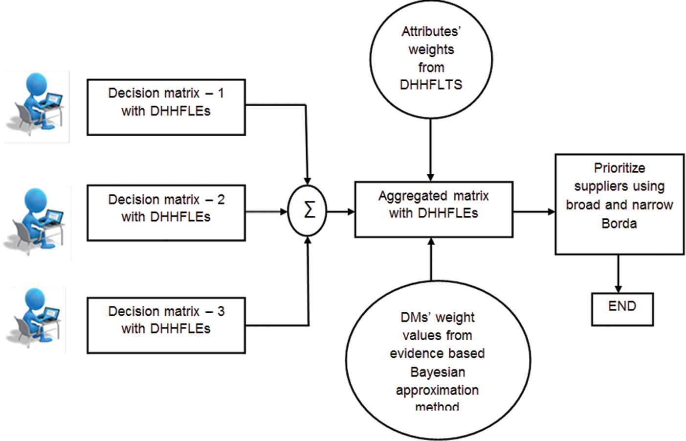
Proposed decision framework.
4. DISCUSSIONS—NUMERICAL EXAMPLE AND COMPARATIVE ANALYSIS
In this section, we put forward a numerical example of green supplier selection for a sports company in India, which clearly demonstrates the practical use of the proposed framework. Further, a comparative analysis is made in this section to realize the strengths and weaknesses of the proposed framework.
4.1. Green Supplier Selection for Sports Company
This section demonstrates the practical use of the proposed decision framework by solving green supplier selection problem for a sports company in India. The company expanded its market widely in India and made a brand-mark in the global market. The company prepared sports accessories like shoes, bands for head and wrist, game kits, etc. The board members wanted to expand their line of focus on jerseys for players involved in the sport. The board members constituted a committee and performed a deep analysis of the pros & cons of the company and prepared an annual report. The board members identified that their contribution to eco-friendly manufacturing was subtle and they needed active eco-friendly practices to compete with the global line-up in a scalable manner. The members found that it was a good idea to start purchasing raw materials from green suppliers who followed green practices actively and are certified by ISO 14000 and 14001. They needed to reframe their purchasing assembly and planned to do the same in a systematic manner.
To do so, the board members constituted a panel of three DMs
Step 1: Begin.
Step 2: Obtain three matrices of order
Step 3: Obtain an attribute weight calculation matrix of order
Tables 1 and 2 provide the data for rational decision-making. Table 1 gives the DMs' preference on each supplier over a specific attribute and Table 2 provides the preference information of a DM on a specific attribute.
| Green Suppliers | Evaluation Attributes |
||||
|---|---|---|---|---|---|
DHHFLE, double hierarchy hesitant fuzzy linguistic element; DM, decision-maker.
Note: For brevity, we directly presented the DHHFLE. For better understanding, the associated linguistic context of
DHHFLEs from DMs.
| DMs | Evaluation Attributes |
||||
|---|---|---|---|---|---|
Note: DM, decision-maker.
Attribute weight calculation matrix.
Step 4: Calculate the attributes' weights by using the matrix in step 3 and the proposed method in Section 3.3.
The DHHFLEs from Table 2 is transformed into a single value by using Eq. (14). Later, Eq. (15) is applied to determine the variance of each attribute. Finally, these variances are normalized by using Eq. (16) and the weight of each attribute is given by (0.03, 0.57, 0.12, 0.16, 0.12).
Step 5: Use the weight vector from step 4 and matrices from step 2 to calculate the weights of the DMs. The procedure in Section 3.2 is used for calculation.
From Tables 3 and 4, we can aggregate the value attribute-wise to obtain
| Green Suppliers (Weighted) | Evaluation Attributes |
||||
|---|---|---|---|---|---|
| (0.112, 0.112, 0.168, 0.112) | (0.446, 0.669, 0.669, 0.892) | (0.591, 0.197, 0.788, 0.394) | (1.195, 0.298, 0.597, 1.195) | (.449, 0.449, 0.449, 0.898) | |
| (0.168, 0.168, 0.224, 0.112) | (0.669, 0.892, 0.892, 0.669) | (0.394, 0.985, 0.788, 0.788) | (0.579, 0.896, 0.896, 0.896) | (0.673, 0.898, 0.898, 0.898) | |
| (0.224, 0.112, 0.112, 0.112) | (0.669, 1.116, 0.892, 0.223) | (0.394, 0.985, 0.985, 0.394) | (0.896, 0.896, 1.195, 1.195) | (0.673, 1.122, 0.449, 0.449) | |
| (0.224, 0.056, 0.168, 0.056) | (0.446, 0.892, 0.669, 0.669) | (0.788, 0.394, 0.394, 0.985) | (0.896, 0.896, 1.195, 0.896) | (0.898, 0.898, 0.673, 0.224) | |
| (0.168, 0.168, 0.224, 0.056) | (0.669, 1.116, 0.224, 0.056) | (0.788, 0.788, 0.985, 0.394) | (0.597, 0.896, 0.896, 0.597) | (0.898, 0.898, 0.673, 1.122) | |
| (0.112, 0.280, 0.168, 0.168) | (0.669, 0.892, 0.892, 0.892) | (0.591, 0.591, 0.788, 0.394) | (0.896, 1.195, 1.494, 0.597) | (0.898, 0.898, 0.898, 0.449) | |
| (0.168, 0.224, 0.224, 0.112) | (0.892, 0.892, 0.669, 0.116) | (0.985, 0.591, 0.788, 0.394) | (0.896, 0.896, 1.195, 0.897) | (0.898, 0.898, 1.122, 0.674) | |
| (0.168, 0.168, 0.280, 0.112) | (0.892, 0.669, 0.892, 0.892) | (0.985, 0.591, 0.591, 0.985) | (1.195, 0.896, 0.896, 0.896) | (0.449, 1.122, 0.898, 0.449) | |
| (0.224, 0.168, 0.168, 0.112) | (0.892, 0.223, 0.446, 1.116) | (0.985, 0.197, 0.591, 0.197) | (0.896, 1.497, 1.195, 1.195) | (0.898, 0.673, 0.673, 0.898) | |
| (0.224, 0.168, 0.224, 0.056) | (0.892, 0.892, 0.669, 0.892) | (0.985, 0.591, 0.591, 0.985) | (0.896, 0.896, 1.195, 1.195) | (0.122, 0.224, 0.898, 0.224) | |
| (0.224, 0.224, 0.168, 0.168) | (0.892, 0.446, 0.669, 1.116) | (0.591, 0.591, 0.985, 0.197) | (1.195, 1.195, 1.494, 0.597) | (0.673, 0.224, 0.898, 0.224) | |
| (0.280, 0.056, 0.056, 0.112) | (0.892, 0.892, 0.892, 1.116) | (0.591, 0.788, 0.788, 0.591) | (1.195, 0.597, 0.597, 1.494) | (0.673, 1.122, 1.122, 0.898) | |
Weighted subscript values.
| Green Suppliers (Normal Bayes) | Evaluation Attributes |
||||
|---|---|---|---|---|---|
| 0.172 | 0.356 | 0.322 | 0.253 | 0.252 | |
| 0.295 | 0.143 | 0.244 | 0.379 | 0.165 | |
| 0.189 | 0.194 | 0.187 | 0.204 | 0.293 | |
| 0.341 | 0.305 | 0.244 | 0.163 | 0.293 | |
| 0.233 | 0.244 | 0.145 | 0.196 | 0.220 | |
| 0.164 | 0.180 | 0.247 | 0.158 | 0.138 | |
| 0.152 | 0.244 | 0.166 | 0.098 | 0.162 | |
| 0.331 | 0.305 | 0.326 | 0.294 | 0.297 | |
| 0.150 | 0.179 | 0.157 | 0.280 | 0.162 | |
| 0.248 | 0.382 | 0.307 | 0.280 | 0.348 | |
| 0.248 | 0.328 | 0.179 | 0.219 | 0.139 | |
| 0.352 | 0.109 | 0.355 | 0.219 | 0.348 | |
Normalized bayes approximation.
The support and creditability measure are calculated using Eqs. (12) and (13) and they are given by
Step 6: The weight vector from step 5 and the matrices from step 2 are used for aggregation. The proposed DHHFMSM operator from Section 3.4 is used for aggregation.
Step 7: Use the aggregated matrix (Table 5) from step 5 to prioritize the green suppliers. Extended Borda method proposed in Section 3.5 is used for prioritization (see Table 6).
| Green Suppliers | Evaluation Attributes |
||||
|---|---|---|---|---|---|
Note: DHHFLE, double hierarchy hesitant fuzzy linguistic element.
Aggregated DHHFLE using DHHFGMSM operator.
| Green Suppliers | Narrow and Broad Borda Count | Ranking |
|---|---|---|
| 9.25 | 4 | |
| 12.75 | 1 | |
| 11 | 3 | |
| 11.25 | 2 |
Ranking using extended Borda method.
Table 5 presents the aggregated value which is used for ranking green suppliers. By the Borda method, we calculate the narrow and broad Borda count and it is shown in Table 6. For narrow Borda,
Step 8: Compare the proposed decision framework with other methods to realize the superiority and weakness. A detailed discussion is made in Section 4.2.
Step 9: End.
These steps are provided for rational evaluation of green suppliers. The main reason is to demonstrate the practical use of the proposed framework. These steps utilize the proposed methods from Section 3 to rationally evaluate green suppliers. Initially, three matrices of order four by five is obtained. Later, a matrix of order three by five is obtained, which is used for calculating attributes' weight vector of order one by five. This vector is used along with three matrices of order four by five to determine DMs' weight vector of order one by three. This weight vector is used to aggregate three matrices of order four by five into a single matrix of order four by five. Finally, Borda method is applied to the aggregated matrix to obtain a vector of order one by four, which is used for prioritizing green suppliers.
4.2. Comparative Analysis: Proposed vs. Others
This section provides a comparative analysis of the proposed framework with other state-of-the-art methods. To maintain homogeneity in the process of comparison, we consider DHHFLTS based MULTIMOORA [14], HFLTS-based MSM operator [30] and multiple HFLTS-based GMSM operator [32]. Table 7 provides the ranking order from different methods and Table 8 provides the analysis of different characteristics of proposed and state-of-the-art methods.
| Green Supplier | Methods |
|||
|---|---|---|---|---|
| Proposed | [14] | [30] | [32] | |
| 4 | 4 | 4 | 4 | |
| 1 | 2 | 2 | 2 | |
| 3 | 3 | 1 | 1 | |
| 2 | 1 | 3 | 3 | |
| Order | ||||
Ranking order: proposed vs. others.
| Factors | Methods |
|||
|---|---|---|---|---|
| Proposed | [14] | [30] | [32] | |
| Data | DHHFLEs | HFLEs | Multiple HFLEs | |
| Aggregation | Yes | No | Yes | Yes |
| Capture interrelationship | Yes | No | Yes | Yes |
| Attribute weight calculation | Yes | No | No | No |
| DMs' weight calculation | Yes | No | No | No |
| Generalization | Followed | No | No | Followed |
| Preference model | Rich and highly flexible | Cannot represent the complex linguistic expression | ||
| Prioritization | Borda method | MULTIMOORA | Aggregation operator-based method | |
| Rank value set | Broad and reasonable | Narrow | ||
| Scalability | Follows Saaty's principle [50] | |||
| Total preorder | Yes | Yes | Yes | Yes |
Note: DHHFLE, double hierarchy hesitant fuzzy linguistic element; HFLE, hesitant fuzzy linguistic element.
Investigation of different factors: proposed vs. others.
From Table 7, we can observe that methods [30,32] produce different ranking order which is mainly due to the loss of potential information from the secondary hierarchy. The proposed method and method [14] use DHHFLTS as preference information and from Figure 2, we can infer that the proposed method is consistent with other state-of-the-art methods. In Figure 2 dhhmultimoora denotes double hierarchy hesitant multiplicative multi-objective optimization by ration analysis, hflmsm denotes hesitant fuzzy linguistic MSM, and mhflmsm denotes multiple hesitant fuzzy linguistic MSM. Figure 2 is a correlation plot, which is formed by calculating the Spearman correlation between ranking orders different methods (proposed and state-of-the-art methods). By applying the Spearman correlation [49] the coefficient values are given by (1, 0.80, 0.40, 0.40) with proposed vs. state-of-the-art methods. From the correlation values it is clear that the proposed framework is highly consistent with [14] and less consistent with [30,32]. The reason can be driven from the fact that [14] uses DHHFLEs (like the proposed framework), but [30,32] use HFLTS information, which causes potential loss of information and hence ranking order is different (for [30,32]) compared to the proposed framework. Hence, it is evident that DHHFLE has potential information to represent complex linguistic expressions, which is lacking in HFLTS. Table 8 presents the characteristics of proposed and other frameworks.
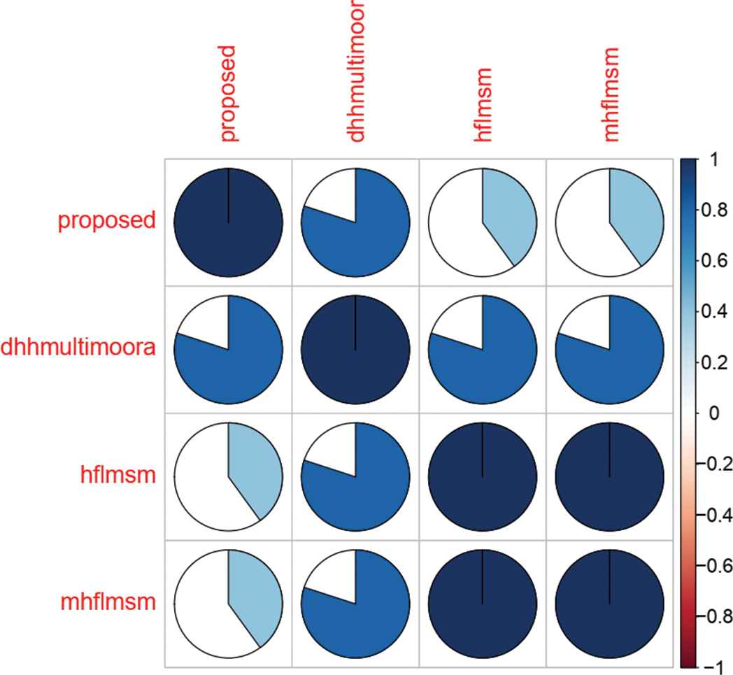
Corrplot of proposed vs. other methods.
Some superiorities of the proposed decision framework are given below:
The DHHFLEs are used as preference information for rating suppliers over a specific attribute. This linguistic model provides a rich and flexible environment for preference elicitation and allows effective representation of complex linguistic expressions.
The hesitation in preference elicitation is properly captured during attributes' weight calculation by using DHHFLTS-based SV method.
Moreover, DMs' weights are calculated in a systematic manner for aggregation of preferences by using evidence theory-based Bayes approximation method.
The matrices from each DM is aggregated in a rational manner by properly capturing the interrelationship between attributes.
From the aggregated matrix, the suppliers are prioritized by using an extended Borda method which produces consistent ranking with other state-of-the-art methods.
The proposed decision framework produces broader and reasonable rank value set which can be effectively used for backup management. To further understand the context, we perform a simulation study in which 300 matrices of order
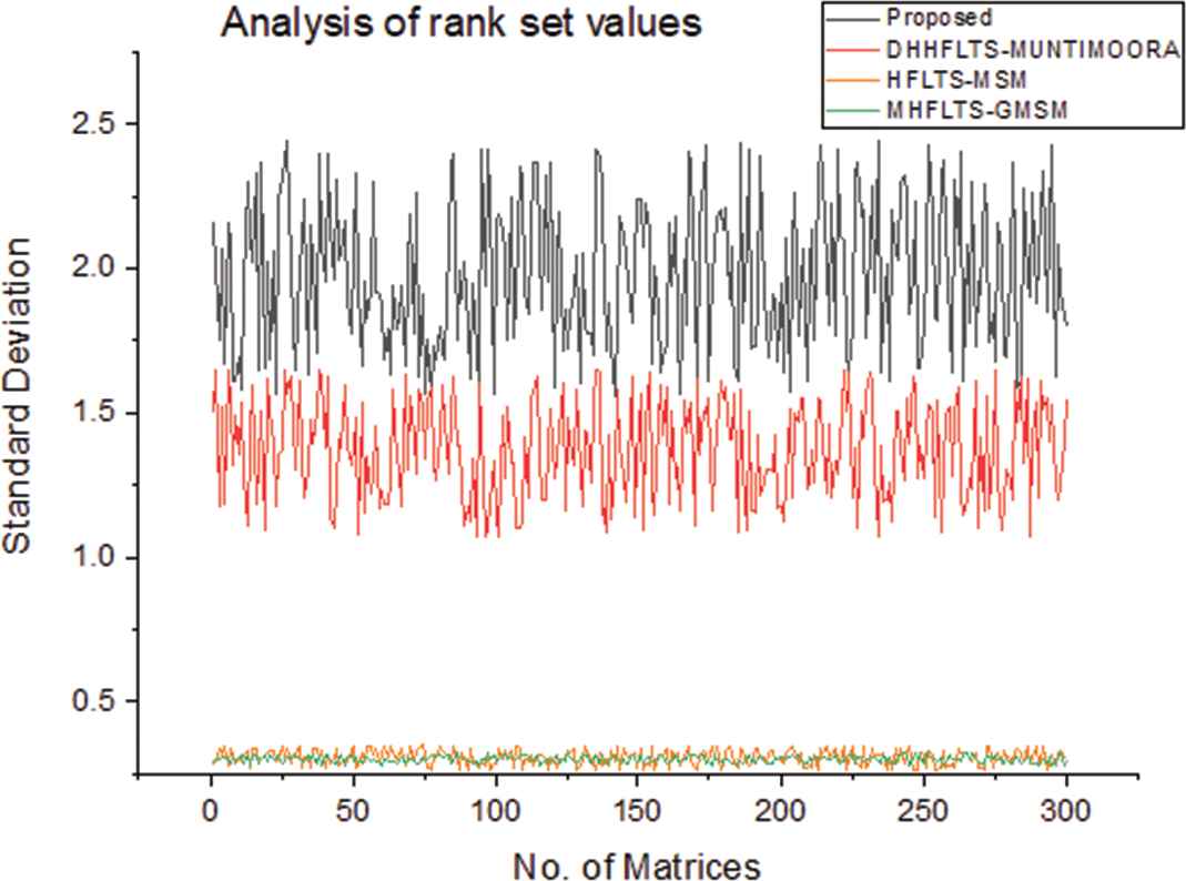
Standard deviation plot: proposed vs. others.
Some limitations of the proposed framework are
DMs need some training with the linguistic model for better understanding the inference. Organization/institutions can conduct hands-on workshops or seminars by inviting experts to train people with the linguistic models and by assignments, they can be evaluated and once people are trained, they can be used for decision-making problems.
Moreover, suitable selection of risk appetite values is needed for effective decision-making. In the future, optimization models can be used for obtaining apt values.
5. CONCLUSIONS
This paper puts forward a new extension to GMSM operator under DHHFLTS context. The DHHFLTS is a rich and flexible linguistic model that provides effective preference elicitation. Moreover, GMSM operator is a generalized form of MSM operator that can effectively capture the interrelationship between attributes. Attributes' weight values are calculated in a systematic manner by properly capturing the DMs' hesitation during preference elicitation. Also, DMs' weight values are calculated in a systematic manner for aggregation of preferences. Later, the Borda method is extended for DHHFLTS context to prioritize objects. The applicability of the proposed decision framework is demonstrated by using a green supplier selection problem and the superiorities and weaknesses of the proposed framework are discussed by comparison with other methods.
Some implications that can be noted are
The framework is a “ready to use” model for making rational decisions. Generally, practical decision problems have attributes that are interrelated and capturing these interrelationships provides rational decision-making.
The DHHFLTS allows effective preference elicitation by providing a rich and flexible environment. Some amount of training is required to adapt to the model.
The framework can be used by the organization for proper planning of purchase and inventory management.
Finally, suppliers can also use the framework to assist their performance and take corrective measures in the required areas of focus.
For future research directions, plans are made to propose new decision frameworks under DHHFLTS context. Also, we plan on integrating recommendation concepts with DHHFLTS-based MADM model. Further, we plan on providing generalized operators for DHHFLEs that could be practically used for rational decision-making.
CONFLICT OF INTEREST
All authors of this research paper declare that, there is no conflict of interest.
AUTHORS' CONTRIBUTIONS
The research was designed and performed by the first and second authors. The data was collected and analyzed by the first and second authors. The paper was written by the first and second authors, and finally checked and revised by the third and fourth authors. All authors read and approved the final manuscript.
ETHICAL APPROVAL
This article does not contain any studies with human participants or animals performed by any of the authors.
ACKNOWLEDGMENTS
Authors thank University Grants Commission (UGC), India and Department of Science & Technology for their financial support from grant nos. F./2015-17/RGNF-2015-17-TAM-83 and SR/FST/ETI-349/2013. Authors also thank the editor and the anonymous reviewers for their constructive comments, which improved the quality of the manuscript.
APPENDIX
| Notations | Meaning |
|---|---|
| Positive integer; upper limit of primary hierarchy | |
| Positive integer; upper limit of secondary hierarchy | |
| Number of alternatives/objects | |
| Number of attributes | |
| Number of DMs | |
| Number of instances in DHHFLE | |
| Index for alternatives/objects | |
| Index for attributes | |
| Index for instances | |
| Index for DMs |
Notations and their meanings.
REFERENCES
Cite this article
TY  - JOUR
AU  - Raghunathan Krishankumar
AU  - Kattur Soundarapandian Ravichandran
AU  - Huchang Liao
AU  - Samarjit Kar
PY  - 2020
DA  - 2020/06/12
TI  - An Integrated Decision Framework for Group Decision-Making with Double Hierarchy Hesitant Fuzzy Linguistic Information and Unknown Weights
JO  - International Journal of Computational Intelligence Systems
SP  - 624
EP  - 637
VL  - 13
IS  - 1
SN  - 1875-6883
UR  - https://doi.org/10.2991/ijcis.d.200527.002
DO  - 10.2991/ijcis.d.200527.002
ID  - Krishankumar2020
ER  -