
A Novel Cause-Effect Variable Analysis in Enterprise Architecture by Fuzzy Logic Techniques
- DOI
- 10.2991/ijcis.d.200415.001How to use a DOI?
- Keywords
- Decision-making; Formal analysis of rules; Enterprise architecture; Fuzzy relation equations; Fuzzy sets
- Abstract
In this paper, we present a new integration approach for managing Information Technology variables within enterprise architecture in an integrated way. Additionially, a novel method based on fuzzy logic for cause-effect variable analysis is proposed as a useful support decision-making tool for companies in order to know the main actions they must perform for increasing their benefits. This is employed to assess the Integration Management System in Enterprises, based on Enterprise Architecture and Information Technology. We show as fuzzy logic plays an important role in this area due to these variables can be affected for multifactorial elements impregnated with uncertainty. The knowledge given by the experts is translated into dependence rules, which have also been analyzed from a fuzzy point of view using a combination of two fuzzy techniques, namely, fuzzy relation equation theory and fuzzy graph. Firstly, fuzzy dependence rules are computed from fuzzy relation equations and, secondly, an analysis based on incidence subgraph is performed. The result is a strategic plan automatically generated from the data captured of each enterprise in which the most import variables to be improved are detailed.
- Copyright
- © 2020 The Authors. Published by Atlantis Press SARL.
- Open Access
- This is an open access article distributed under the CC BY-NC 4.0 license (http://creativecommons.org/licenses/by-nc/4.0/).
1. INTRODUCTION
Nowadays, analytics (data and variable analysis) provide competitive advantages for companies. In fact, Forbes has established that companies that still are not investing heavily in analytics by 2020 probably will not be in business in 2021 [1]. This is due to the great opportunities associated with data and variable analysis for helping companies to get a better understanding of the market and make timely business decisions [2]. At the same time, enterprises need data and variable analysis in order to assess their developments, improvements and achievements. The obtained knowledge will allow them to increase their benefits.
On the other hand, one of the most important problems detected in companies is the necessity of integrating in pursuit of a common goal. The lack of this integration weakens the companies, generating discontent and recurrent problems both internally and externally, creating barriers for the effective fulfillment of the mission and the vision [3,4]. The use of new technologies is also important to increase the efficiency and effectiveness levels in a company.
The integration of a management system for enterprises throughout strategic management models associated with enterprise architecture (EA) is an important contribution of this work since the current management models do not consider Information Technology (IT) variables in an integrated way. Integration Management System in Enterprises (IMSE) aims this integration from different points of view and, in particular, with the use of IT, throughout strategic management models associated with EA. EA is an important research field in the business sector, which has several approaches: the alignment approach, focuses on interconnect the organization's strategies with IT in order to achieve greater performance [5–7]; the system approach, aims at the holistic representation and coherent distribution of organizational levels in the processes, information systems and technological infrastructure [8,9]; the strategic approach, which describes a current stage of the organization through the interconnection level of the processes, the ITs and the strategies, and leads to a future stage or higher level of maturity by using, for example, frameworks, models and tools adapted to different business contexts [10–12]. This model has emerged as a theoretical and practical response to the shortcomings in the field of strategic management with respect to the strategic direction that organizations should take toward the future, taking full advantage of their capabilities, based on a coherent and coordinated relationship between all key and functional processes and external entities [3].
For all these reasons, data and variable analysis in the EA is an important and mandatory tool for companies because it allows them to assess the IMSE, based on EA and IT. As a consequence, the enterprises will have a supporting decision-making mechanism in order to know the main actuations they must perform for increasing their benefits, based on the assessment of EA variables. In this paper, analytics is applied to EA discipline.
Emerging analytics research can be classified into five critical technical areas: data analytics, text analytics, web analytics, network analytics and mobile analytics [2]. AI and machine learning become force multipliers for data analytics. One of these techniques is the well-known path analysis (PA) paradigm which aims to asses theoretical models in which a set of dependencies relations between variables is proposed. A new mechanism based on fuzzy logic for assessing a strategic management model is proposed in this paper. This method is based on five phases:
Definition of variables. In this phase, the main variables together with the relations among them are established and obtained from a study of the EA literature and prestigious EA experts.
Stages and dependences among the variables. In this phase the different variables in EA are analyzed from a theoretical point of view, in order to provide the IMSE model. As a consequence, diverse cause-effect relations, existing among the introduced EA variables, are established. The considered variables are grouped in three stages (identified with 5, 12 and 5 variables each one) by taking into account the strategic management processes presented in an organization.
Collect and store observations. Particular values for each variable are obtained from a questionnaire which is answered by a set of experts. The questionnaire is based on a checklist with options between 0 and 1. The checklist is designed by taking into account theoretical analysis of variables for EA and the semantic relations between variables and the correlations established between them (see Example 1).
Fuzzy decision rules analysis. In this phase, dependences are represented as fuzzy decision rules, in which the weights are unknown. In order to compute that weights, different equations arise and so, fuzzy relation equations (FREs) theory [13] is applied to solve them [14–16]. The weight of each rule shows the truth value of the rule, that is, the (observed) real relationship between the variables in the rule. Hence, we can check whether the theoretical dependence is supported by the observations and if this relation should be changed or removed.
Priority strategy based on the incidence graph. The development of this set of fuzzy dependence rules also provides a variable prioritization mechanism, that is, offers the most important variables to be improved when the EA needs improvements. In order to do that, a procedure for computing a priority value to each variable, based on the incidence of the variable in the rest of variables of the stage is performed. Specifically, for each variable, all directed paths from this to a final variable will be generated and its associated degree will be computed.
This method has been applied to different Cuban enterprises obtaining good results and providing an effective mechanism to improve the IMSE [17]. This paper aims to strengthen the theoretical study from the observed data of the different considered companies. In order to have a set of heterogeneous data, companies from diverse sectors have been taken into account, such as construction, biopharmaceutical, communications, real estate and tourism sector. If the company has a limited budget to increase the IMSE, with this mechanism the company can focus its efforts on the prioritized variables, whose enhancement also increases other important variables, optimizing the resources and increasing the benefits.
The structure of the paper is as follows: Section 2 recalls the main notions of FREs, Section 3 presents the strategic management model with an EA approach for the IMSE and also details the cause-effect relations (variables grouped in three stages), relations—cause, effects—among them and the definition of rules by using logic implications. In Section 4 dependencies analysis between variables based on fuzzy logic is explained. In Section 5 an evaluation by using priority strategy based on incidence graphs is performed. Finally, diverse conclusions and prospects for future work are included.
2. FUZZY RELATION EQUATIONS
The FREs were introduced by E. Sanchez [18] as a mathematical tool based on the composition of fuzzy relations and focused on solving medical problems. From its introduction, FRE has been developed in theoretical and practical aspects. For instance, FRE has also been considered in approximate reasoning, automatic control or decision-making.
Given a set
Different algebraic structures have been considered to define the composition of fuzzy relations. For example, the first composition considered the maximum and the minimum on the unit interval [18]. Recently, more flexible operators have been considered [15,16,19], which have a better adjustment to real cases. For example, the structure considered in [16] will be recalled in this section to be used later.
Given a complete lattice
Given an adjoint pair
The solvability of these equations was also studied in [16], obtaining that a FRE
In the study presented in this paper, for illustrating the given procedures, we will consider the lineal lattice
3. EA TO STRATEGIC MANAGEMENT
The Strategic Management model focuses on the EA to get a complete Integration Management System in the Enterprise (SMEA-IMSE), considered in this paper, is based on IMSE and aims to improve the level of integration of the management system of the enterprise by using the variables of EA and strategic management.
This model is based on the main ISDE approaches: strategic, client-oriented and processes [21], together with a new approach based on EA. The main properties are the following:
Integration. All management elements of the EA are analyzed in order to determinate which of them are important for the external and internal relationships.
Teamwork. The model is implemented by a team of experts, which is leaded by the manager of the company, together with the personal involved in the different stages of the processes.
Predictability. It offers tools for making preventive and flexible decisions within the management system.
The implementation of the model initially requires compliance with several fundamental premises:
The processes and flows of the generated information must be defined and identified.
The senior managers in the company must feel committed with the proposed changes.
The company must have at least one defined strategic plan and work according to the goals reflected in it.
The IT must be involved in the strategic plan. IT must be a key element in the strategic plan and its involvement and development must be assessment.
3.1. Design of the SMEA-IMSE
Now, we will present the main variables of the EA we have detected, and the relations among them, which have been obtained from a study of the EA literature and prestigious EA experts [17,21]. As a consequence, diverse cause-effect relations, existing among the introduced EA variables, have been established.
The considered variables are grouped in three stages by taking into account the strategic management processes presented in an organization. The relation between EA and Strategic Management has been discussed in previous papers [17,22]. For each stage two steps will be carried out:
Definition of variables and cause-effect relations among them.
Quantification of them and definition of the rules.
3.1.1. Stage 1
Process-Based Strategic Design (PSD) is the first stage and is focused on determining the strategic direction of the organization, taking into account mainly the results of the integration level of the enterprise management system and the internal and external strategic diagnosis. The variables involved in this phase are
Strategic Team (ST,
Communication among Stakeholders (CS,
Strategic Project (SP,
Diagnosis, Design and Redesign of the Key Processes (DDRKP,
Diagnosis, Design and Redesign of the Functional Processes (DDRFP,
From these variables the theoretical study determines diverse cause-effect relations among them (see Figure 1), which dependences are represented as follows:
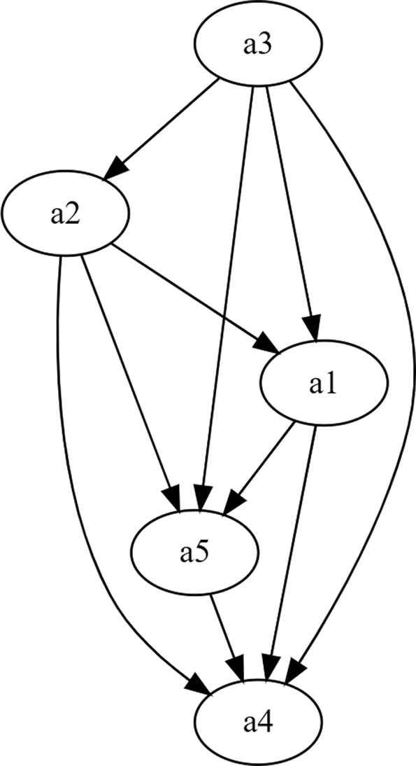
Diagram established between the variables involved at Stage 1.
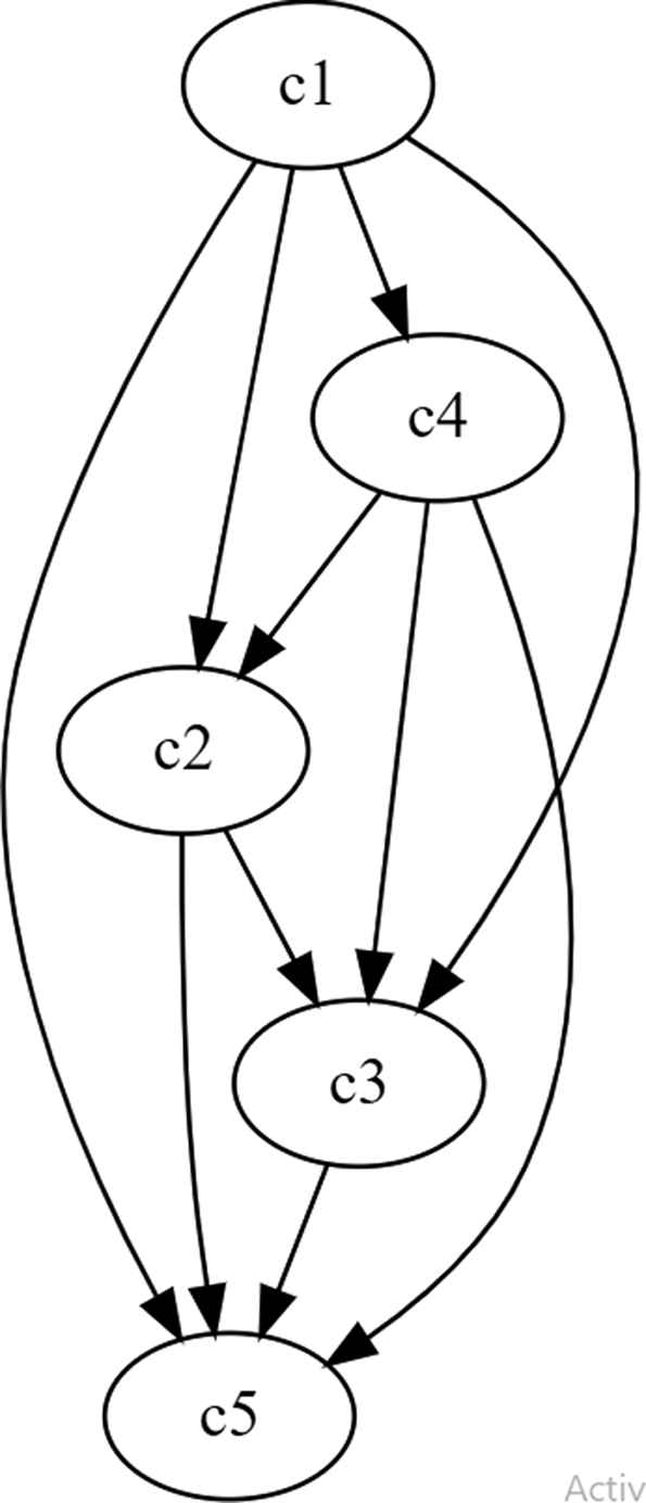
Relations established between the variables involved in Stage 3.
For example, the first dependence should be read as follows:
3.1.2. Stage 2
Strategic Design based on the Approach of the EA. This second stage aims to provide solutions based on EA and focusing on the key, strategic and low performance support processes within the corporate system. The variables involved in this stage are
Technological Vigilance (TV,
Management and Automation of processes (MA,
Response Capacity (RC,
Management of Relevant Information in processes (MRI,
Information Security (IS,
Integration of Information for strategic decision-making (II,
Structure of IT Applications (SA,
Interoperability of IT Applications (IA,
Exploitation of IT Applications in Key processes (EAK,
Investments in Technological Infrastructure (ITI,
Exploitation of Technological Infrastructure (ETI,
Integration Technological infrastructure and IT Applications (ITA,
In this stage, the established cause-effect relations are the following:
3.1.3. Stage 3
Implementation, Control and Supervision is the last stage and aims to optimize the model proposed using the strategic plan and a set of actions based on EA. The variables involved in this stage are
Leadership (L,
Assimilation of Changes by the workers (AC,
Management of Efficiency and Effectiveness Indicators (EEI,
Integration of IT with Strategic Objectives and processes (ISO,
Generation of Value (GV,
Hence, a total of five variables are considered and the theoretical study has determined the following cause-effect relations:
3.2. Strategic Technological Capacity and Dataset of Observations
The strategic TEchnological CApacity (TECA) is the main indicator of the strategic management model SMEA-IMSE, which is associated with a specific company. TECA is defined as the ability to manage the design, implementation and control of a strategic project for the integration of the management system of the considered company, throughout EA variables. TECA is computed from the previous set of variables, grouped in the three phases:
Process-Based Strategic Design
Strategic Design based on the Approach of the EA
Implementation, Control and Supervision
For each company to be studied, this indicator is computed from the particular values obtained from a checklist that the experts of the company have filled in and the set of cause-effect relations given above [17,21]. These managers and/or specialists of different real companies have answered different questions in the checklist we have prepared for assessing all variables. The questions have a score (with a value between 1 and 10) and they have been aggregated using the geometric measure for computing the TECA. The details of this checklist and the considered procedure are given in [23,24]. Next, an example of question is presented.
Example 1.
For example, for the Strategic Project variable (question 1.3 in the checklist [24], which has been summarized in order to be more concise in this paper), the expert must answer the following question: is the Strategic Projection being developed efficiently by the organization? For what the expert has the following options:
Not, it is not being developed (0).
Yes, a strategic projection for the organization is carried out. Very few objectives are achieved (0.1, 0.2, 0.3).
Yes, a strategic projection for the organization is carried out. Some objectives are achieved (0.4, 0.5, 0.6).
Yes, a strategic projection for the organization is carried out. Many strategic objectives hold (0.7, 0.8, 0.9).
Yes, a strategic projection for the organization is carried out by using ITs. The strategic projection is updated quarterly, this guarantees the fulfillment of all proposed strategic objectives (1).
The following example shows a set of values obtained from a checklist that an expert fills. These values are stored in a dataset of observations, which will be fundamental for the next step (Section 4).
Example 2.
For example, for each stage, an expert will establish a score for company
Stage 1:
Stage 2:
Stage 3:
Therefore, in order to compute an efficient and proper TECA for the companies, it is very important to analyze and assess the cause-effect relations obtained from the literature and experts in order to be sure that they correctly hold in the practical cases. This complementary study is introduced in the Section 4, which will be based on the stored dataset.
4. COMPUTING FUZZY DEPENDENCE RULES FROM FRE
The established cause-effect relations existing among the variables, in each stage, have been obtained from a theoretical study of EA literature [17, 21], as previously was commented. Hence, in order to complement this study, it is fundamental to consider another mechanism that assess the obtained set of cause-effect relations. The selected mechanism is the application of FREs, due to its relation to decision-making and fuzzy dependence rules [14,20], and that the real data does not form a big dataset.
In this section, the dataset obtained from experts (managers and specialists) of several real companies will be considered in order to compute a truth value (weight) to each crisp cause-effect relation given by the theoretical study of the EA literature. As a consequence, fuzzy dependence rules will be obtained, in which the weight of each rule will show its relevance. This truth value will be computed making use of the FREs and the obtained rules will be compared with the crisp ones.
Specifically, from the crisp dependences, a set of fuzzy dependency rules is obtained. Each rule is formed by a head, a body and its corresponding weight, that is,
In [14,20], the authors proved that, given a set of rules:
Specifically, from the instantiations of each (effect and cause) variable given by the checklists of each company, a matrix is obtained. This matrix will be used, together with the set of cause-effect rules established in the theoretical framework, to define a FRE. The solutions of this equation will provide the weights (truth values) of these rules.
Notice that, these weights can be interesting for assessing the validity of such rules and for measuring the plausibility of the data observed in future cases. Moreover, these weights can also offer the possibility of providing a priority among the causes of a certain effect, which is very important when the company wants to solve or improve its productivity and/or strategic management. The computed priority will suggest what cause should be improved (increasing its value) firstly in order to increase the effect more quickly. Therefore, if an effect needs to be improved, this priority provides what modification in the values of the causes influences more in the final value of the effect and so, we can optimize the resources given to boost the effects.
In order to design an heterogeneous real data set, six companies from different sectors, sizes and characteristics, are considered. They have been denoted as
| Variable | ||||||
|---|---|---|---|---|---|---|
| 7.56 | 6.26 | 2.25 | 3.17 | 7.81 | 6.22 | |
| 6.44 | 6.26 | 3.91 | 4.80 | 15.64 | 7.60 | |
| 8.78 | 7.19 | 4.20 | 5.23 | 7.59 | 7.82 | |
| 9.00 | 6.32 | 3.10 | 5.30 | 7.66 | 8.02 | |
| 8.78 | 6.16 | 3.83 | 3.88 | 7.70 | 7.63 |
Input matrix for Stage 1.
| Variable | ||||||
|---|---|---|---|---|---|---|
| 8.00 | 6.22 | 4.29 | 3.01 | 7.83 | 7.12 | |
| 7.22 | 7.43 | 4.14 | 4.94 | 6.93 | 4.95 | |
| 7.56 | 5.11 | 3.24 | 3.36 | 6.46 | 5.87 | |
| 7.00 | 5.18 | 2.98 | 3.56 | 6.80 | 5.02 | |
| 7.89 | 5.74 | 3.23 | 4.74 | 8.25 | 8.12 |
Input matrix for Stage 3.
| Variable | ||||||
|---|---|---|---|---|---|---|
| 6.89 | 6.02 | 3.56 | 3.20 | 5.07 | 7.14 | |
| 6.89 | 7.08 | 3.82 | 3.99 | 5.21 | 6.82 | |
| 6.56 | 6.55 | 2.36 | 2.70 | 6.81 | 7.78 | |
| 8.78 | 7.21 | 3.11 | 3.58 | 6.23 | 7.83 | |
| 6.89 | 8.34 | 5.73 | 5.50 | 6.32 | 8.47 | |
| 7.22 | 7.18 | 3.64 | 3.79 | 6.96 | 7.84 | |
| 8.33 | 6.78 | 4.28 | 4.92 | 7.96 | 7.95 | |
| 5.67 | 5.96 | 1.97 | 4.33 | 6.68 | 4.84 | |
| 7.11 | 6.54 | 3.56 | 4.03 | 5.64 | 6.64 | |
| 8.11 | 7.20 | 3.70 | 4.55 | 6.26 | 4.13 | |
| 7.78 | 7.50 | 3.04 | 4.20 | 6.68 | 6.40 | |
| 7.22 | 7.69 | 2.42 | 4.55 | 5.82 | 5.38 |
Input matrix for Stage 2.
Next, the procedure will be illustrated for the rules associated with a given variable. Specifically, the effect
The submatrices
From the theory of FREs, we know that, if
As a consequence,
The nonsolvability character of the system can be given by the inherent uncertainty of the answers of the experts, the computation error, etc. Hence, although the equation could have some solution, it is not possible to obtain the exact solution. For that cases, Cornejo et al. introduced in [20] two approximation mechanisms. In this paper, the pessimistic/conservative approximation is adapted to the considered problem.
This optimal approximation considers the values of
Therefore, since these true values are high, we can say that the truth values obtained from the application of FRE to the data provided by experts are very close to those established from the theoretical point of view.
Since these truth values show how the cause variables increase the performance of the EA, another important consequence of the computation of these weights, as we previously commented, is that a priority among the variables can be given to improve the TECA. For example, if the manager of the company wants to improve the value of the effect variable
The procedure is applied to every variable in every stage and all the weights are computed. The complete list of weighted rules are given in Tables 4 and 5. These weights complement the diagram (direct graph) in Figures 1–3. The obtained weighted directed graphs are presented in Figures 4–6, respectively.
| Stage 1 | Stage 3 |
|---|---|
Fuzzy dependencies rules for Stages 1 and 3.
| Stage 2 |
|---|
Fuzzy dependencies rules for Stage 2.
These graphs provide very interesting information, for example, we can extract from them what variables are more causes and what variables are more effects. For example, in Stage 1, the variable with less incidence in the rest is the variable
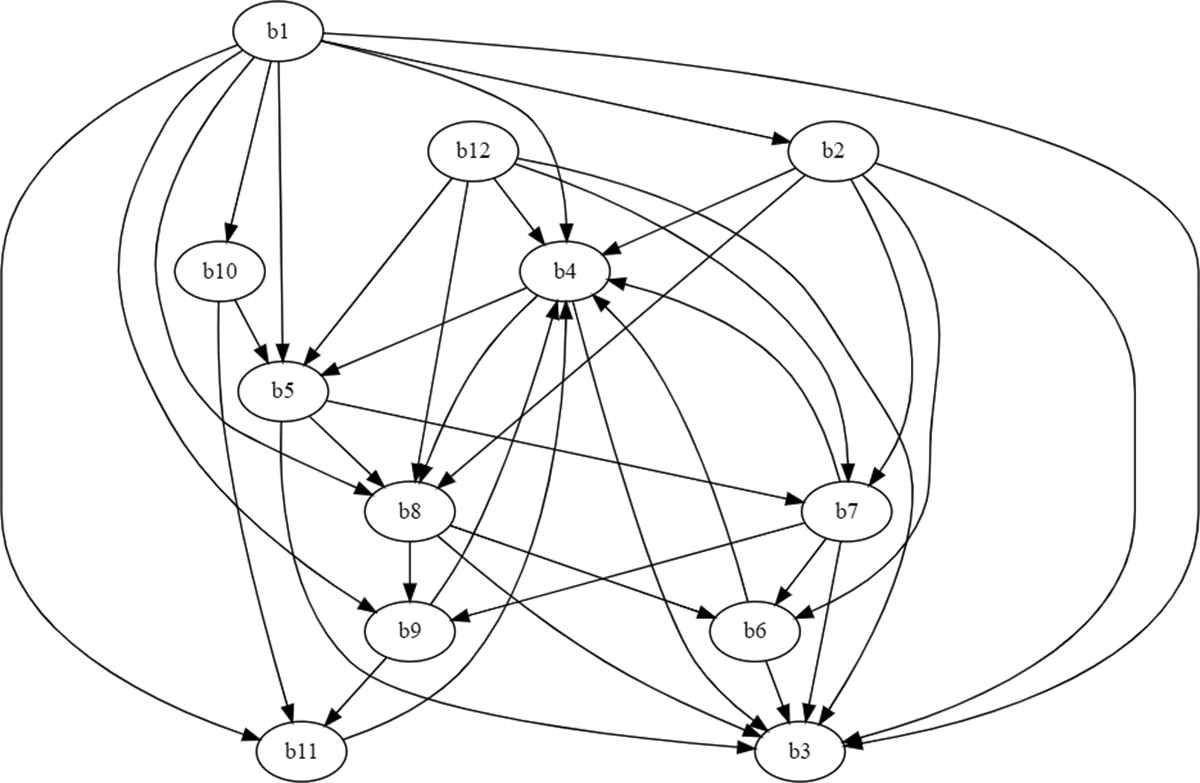
Relationship between the variables of Stage 2.
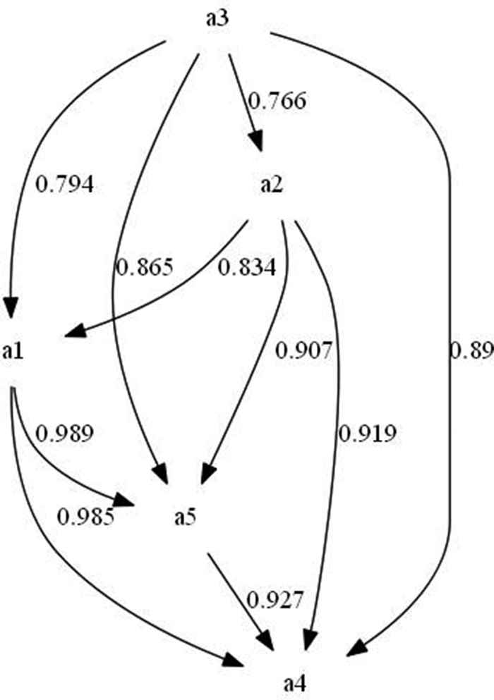
Relations established between the variables involved in Stage 1 and the weights computed by each one of them.
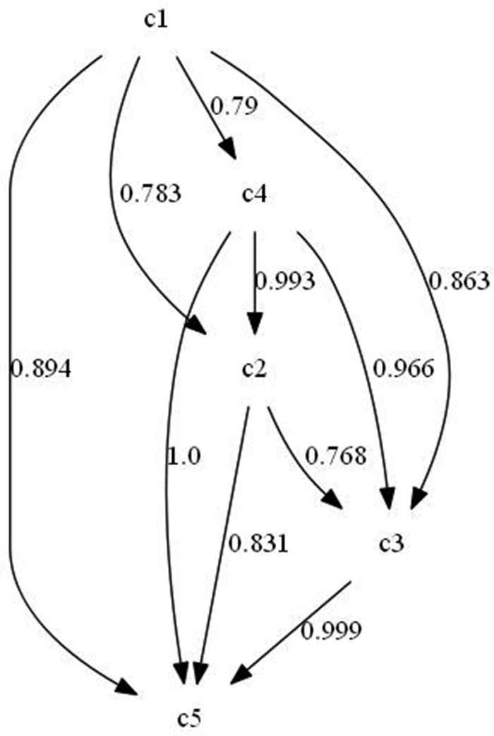
Relations established between the variables involved in Stage 3 and the weights computed by each one of them.
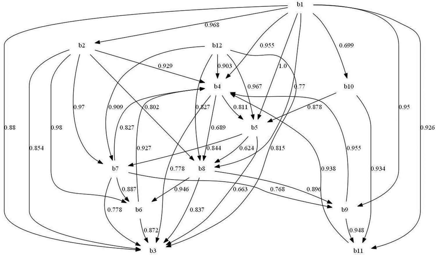
Relations established between the variables involved in Stage 2 and the weights computed by each one of them.
Hence, if for a particular company, the value of the variable
Concerning the rest of variables, we can believe that the second most important variable is
Stage 3 also involves few variables and relations and similar strategies of priority can be established. We can see that the variable with less incidence in the rest is
The relations established between the variables involved in Stage 2 are more complex and the computed weights also provide experts useful information about the cause-effect relations. As it can be observed, the variable with less incidence in the rest is the target (cause) variable
5. PRIORITY STRATEGY BASED ON THE INCIDENCE GRAPH
This section will introduce a procedure for computing a priority value to each variable, based on the incidence of the variable in the rest of variables of the stage. Specifically, for each variable, all directed paths from this to a final variable are generated and its associated degree is computed. The first step will be to compute the local impact of every vertex.
5.1. Local Impact of Vertices
For correcting the possible deficiencies detected by the indicator TECA for a particular company, it is important to know what variable must be improved and it is also fundamental to know the incidence of each variable in it. Therefore, we also need to know the incidence of each variable in the rest of variables of every stage. Before formally introducing this notion, we need the following two definitions.
Definition 1.
Given a set
From the weights considered in a path, a degree associated with the path can be computed.
Definition 2.
Given a weighted directed graph
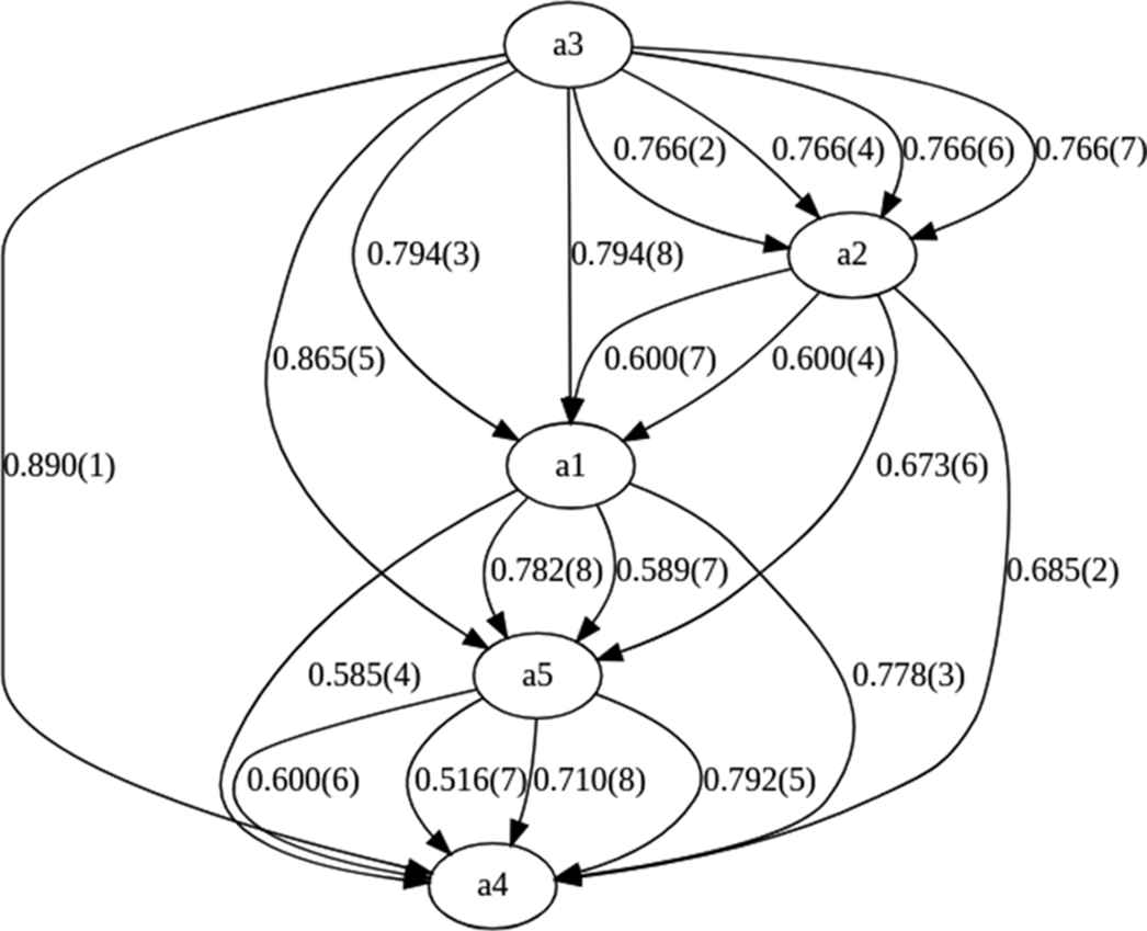
Hence, the associated degree is obtained applying a t-norm to all the weights in the path. The operator considered for the examples is the Łukasiewicz conjunction, which is the same operator considered in the resolution of the FRE in Section 4. Table 6 shows all paths and associated weights from
| Source | Target | Path | Degree |
|---|---|---|---|
| a3 | a2 | 0.766 | |
| a3 | a1 | 0.794 | |
| a3 | a1 | 0.600 | |
| a3 | a5 | 0.865 | |
| a3 | a5 | 0.673 | |
| a3 | a5 | 0.782 | |
| a3 | a5 | 0.589 | |
| a3 | a4 | 0.89 | |
| a3 | a4 | 0.685 | |
| a3 | a4 | 0.778 | |
| a3 | a4 | 0.585 | |
| a3 | a4 | 0.792 | |
| a3 | a4 | 0.600 | |
| a3 | a4 | 0.516 |
Path degrees for the source variable
When several paths arise for the same final variable, the maximum degree of the different paths is computed in order to know the real impact from the source variable to the target one.
Definition 3.
Given a weighted directed graph
In the computation of the impact, the maximum operator collects the useful information, since it shows the most efficient path to be considered in the computation of the influence between two vertices. For example, given the variable
Figures 7 and 8 present the different paths with different kind of lines (continue, dash, etc.), from
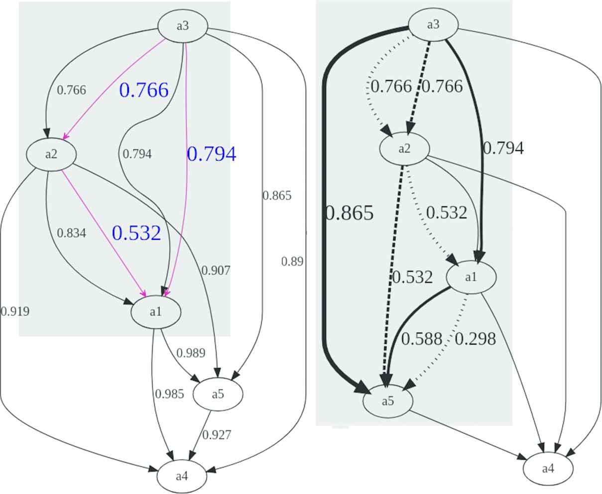
Incidence subgraph of the variable (right).
Incidence subgraph of the variable.
From these paths, the maximum value is computed for each pair
| Source | Target | Path | Impact of |
|---|---|---|---|
| a3 | a2 | 0.766 | |
| a3 | a1 | 0.794 | |
| a3 | a5 | 0.865 | |
| a3 | a4 | 0.89 |
Fuzzy incidence of
Notice that
5.2. Relationship with the Fixed-Point Semantics
We need to take into consideration that the set of rules given for each stage and detailed in Tables 4 and 5 are fuzzy logic programs [26–28], which can be denoted as
Therefore, in order to obtain deductions and consequences from observed values (facts) an operational semantics procedure can be applied, such as the one given by the fixed point semantics [25,29], which is based on the immediate consequences operator. Next, only the definition of this operator will be recalled, the details of this theory can be checked in [26,30].
Definition 4.
Let
From this operator, it is well-known that the consequences arise from the least model of the program, which coincides with the least fixed point of
Notice that, the vertices of the associated directed graph
Theorem 1.
Given an adjoint pair
Proof.
Given
As a consequence, if
Thus, by the associativity of
Since this procedure can be applied to all
As a consequence, the computation of the least model on a propositional symbol (vertex) depends on the impacts of the rest of vertices on it. Therefore, this result really justifies that
5.3. Global Impact of Vertices
It is also very interesting to know a global impact indicator of the variables involved in every stage. This indicator will be given from the sum of the appropriate impact to the rest of variables.
Definition 5.
Let
Another interesting factor is the “quality” of this influence, how big this influence is. This degree is obtained normalizing the FID, that is, computing the average of the FID with the number of target variables.
Definition 6.
Given a weighted directed graph
These last values/indicators provide fundamental information with respect to the global and normalized impact that a variable has in the rest of variables of the stage. Tables 8–10 show these values for the three stages. These figures also include the crisp priority observed in the previous section, the degrees FID and NFID. These last values provide a global priority (FID), which coincide with the crisp priority in Stages 1 and 3, and improve the priority in Stage 2, and a normalized priority (NFID), which shows a better ordering of the variables to be improved, if we are focused on a specific goal variable, only considering the variables involved in the incidence graph of this fixed variable. For example, if we want to improve variable
| Variable | Crisp Priority | FID | NFID |
|---|---|---|---|
| a3 | 4 | 3.315 | 0.828 |
| a2 | 3 | 2.66 | 0.886 |
| a1 | 2 | 1.978 | 0.989 |
| a5 | 1 | 0.927 | 0.927 |
| a4 | 0 | 0.0 | 0.0 |
FID, fuzzy incidence degree; NFID, normalized fuzzy incidence degree.
Crisp priority, FID and NFID of Stage 1.
| Variable | Crisp Priority | FID | NFID |
|---|---|---|---|
| c1 | 4 | 3.337 | 0.834 |
| c4 | 3 | 2.985 | 0.995 |
| c2 | 2 | 1.599 | 0.7995 |
| c3 | 1 | 0.999 | 0.999 |
| c5 | 0 | 0.0 | 0.0 |
FID, fuzzy incidence degree; NFID, normalized fuzzy incidence degree.
Crisp priority, FID and NFID of Stage 3.
| Variable | Crisp Priority | FID | NFID |
|---|---|---|---|
| b1 | 8 | 10.936 | 0.994 |
| b2 | 5 | 8.780 | 0.975 |
| b12 | 5 | 8.604 | 0.956 |
| b7 | 4 | 6.916 | 0.864 |
| b4 | 3 | 5.555 | 0.793 |
| b8 | 3 | 5.567 | 0.927 |
| b5 | 3 | 3.439 | 0.688 |
| b6 | 2 | 3.215 | 0.803 |
| b9 | 2 | 1.896 | 0.948 |
| b10 | 2 | 1.868 | 0.934 |
| b11 | 1 | 0.875 | 0.875 |
FID, fuzzy incidence degree; NFID, normalized fuzzy incidence degree.
Crisp priority, FID and NFID of Stage 2.
6. CONCLUSIONS AND FUTURE WORK
In this paper, a strategic management model has been proposed which allows companies to evaluate EA variables as an IT management approach and to contribute to the IMSE, which has been the first goal of the paper. For assessing this model, we have used the called strategic TECA indicator which provides organizations with the ability to manage the design, implementation and control of a strategic project for the integration of the management system of the considered company, throughout EA variables. The different variables needed in the design of the EA have been selected, classified and related following a theoretical study.
For each company to be studied, this indicator is computed from the particular values obtained from a check-list that the experts of the company fill in and the set of cause-effect relations given above. In this process, cause-effect relations defined between variables and obtained from the literature and experts are analyzed and evaluated in order to be sure that they correctly hold in the practical cases. Additionally, a method for assessing interrelated variables of EA in a strategic management model based on integration theory of management systems in enterprises has been presented and detailed. It can be seen as a novel cause-effect variable analysis method for Integration Management Systems in Enterprises which employs fuzzy logic techniques: fuzzy dependence rules has been obtained by making use of the FREs; we have shown as these weights can be interesting for assessing the validity of such rules and for measuring the plausibility of the data observed in future cases. In particular, the relations given by the theoretical study have been checked considering fuzzy decision rules, computing the weights of these rules and highlighting the most important relationships. These fuzzy rules have also been fundamental for providing a priority in the variables to be improved when the indicator TECA of the IMSE of the company needs to be improved.
Specifically, we have shown how these weights can also offer the possibility of providing a priority among the causes of a certain effect, which is very important when the company wants to solve or improve its productivity and/or strategic management. Therefore, if an effect needs to be improved, this priority provides what modification in the values of the causes influences more in the final value of the effect and so, we can optimize the resources given to boost the effects.
Thus, FREs, fuzzy rules and incidence graphs have been considered to the second main goal of the paper, that is, providing an effective mechanism to improve the IMSE of the companies.
In the future, other complementary tools will be considered, such as fuzzy logic programming, which can be used for analyzing the approximate solution given by the FRE and the possible loops in the (incidence) graphs. Other interesting tool is Fuzzy Cognitive Maps, since they can also be useful for handling cicyles. Furthermore, since the introduced mechanism is portable, that is, it does not depend on the country of the companies, it will be applied to other real companies in Europe and other continents.
CONFLICT OF INTEREST
The authors declare no conflicts of interest.
Funding Statement
Partially supported by the State Research Agency (AEI) and the European Regional Development Fund (FEDER) project TIN2016-76653-P and by the European Cooperation in Science & Technology (COST) Action CA17124.
ACKNOWLEDGMENTS
The author would like to thank the anonymous referees for their careful reading of the paper and useful suggestions to clarify this work.
REFERENCES
Cite this article
TY  - JOUR
AU  - C. Rubio-Manzano
AU  - Juan Carlos Díaz
AU  - D. Alfonso-Robaina
AU  - A. Malleuve
AU  - Jesús Medina
PY  - 2020
DA  - 2020/05/02
TI  - A Novel Cause-Effect Variable Analysis in Enterprise Architecture by Fuzzy Logic Techniques
JO  - International Journal of Computational Intelligence Systems
SP  - 511
EP  - 523
VL  - 13
IS  - 1
SN  - 1875-6883
UR  - https://doi.org/10.2991/ijcis.d.200415.001
DO  - 10.2991/ijcis.d.200415.001
ID  - Rubio-Manzano2020
ER  -