
A Two-Stage Multi-objective Programming Model to Improve the Reliability of Solution
- DOI
- 10.2991/ijcis.d.200410.001How to use a DOI?
- Keywords
- Multi-objective programming; Randomness; Expectation value; Fuzzy events; Reliability
- Abstract
Randomness is a common uncertainty encountered in practical multi-objectives decision-making. But it is always a challenge for decision-makers to process randomness in multi-objective programming problems. This paper takes the decision-making objectives as fuzzy events and aims to solve numerical multi-objective programming problems under random environment. We first analyze the effects of randomness on multi-objective decision-making results. With the expectation value and the probability of fuzzy events as quantitative index of randomness, we then establish a two-stage random multi-objective programming model based on reliability (i.e., TS-MOPM). Specifically, we give several probability calculation methods of fuzzy events with common distributions, and further present the corresponding calculation procedures for solving TS-MOPM. Finally, a case study is implemented to test the proposed model TS-MOPM. Theoretical analysis and case study indicate that our model has better interpretability and operability. The research results enrich the existing random multi-objective programming methods to some extent.
- Copyright
- © 2020 The Authors. Published by Atlantis Press SARL.
- Open Access
- This is an open access article distributed under the CC BY-NC 4.0 license (http://creativecommons.org/licenses/by-nc/4.0/).
1. INTRODUCTION
In today's real world, complexity has considerably raised for decision-makers because of the increasing uncertainties they are facing. A variety of decision-making problems often involve various objectives to be achieved at the same time. For example, water quality planning and management may refer to factors such as the implementation levels, unit costs, reduction efficiency and total pollution loads [1,2]; emergency relief management considers several different objectives as logistics time, logistics costs, the amount of unsatisfied demand, service delays, the ability of sustainable rescue [3,4]; transportation network should balance three indices transportation cost, transportation time and emissions to optimize the system performance [5]; agricultural water and land optimization allocation is a complicated problem involving many objectives [6]; suppliers selection in supply chain management involves some objectives such as cost minimization, the quality of raw materials, on-time delivery and sustainability [7]. In view of the above applications, a multi-objective optimization is the most potential way. Thus, modeling real life problems as formulated multi-objective programming and further giving corresponding solution are two main concerns in management field.
Multi-objective programming is an optimization problem characterized by a set of objective functions and a set of well-defined constraints to be satisfied [8–10]. The goal of multi-objective programming is to identify all the feasible solutions in which it is impossible to optimize the value of one objective function without making the value of at least one other objective worse [11]. Charnes et al. [12] firstly established a multi-objective linear programming model based on bias variables by introducing positive and negative deviation variables and priority factors (including rank and weight). More information on multi-objective programming can be referred to Ehrgott [9,13].
Because many practical decision-making problems can be formulated as a multi-objective programming, the wide application spectrum and ever-increasing strong interests have encouraged the substantial development of reliable models and efficient algorithms during the recent decades [14–17]. Numerous researches have been devoted to multi-objective programming combining with different theories and methods, and many significant theoretical and applied findings have been also achieved. Han et al. [16,17] discussed the solution to multi-objective programming with hierarchical structure (bi/tri-level decision-making). Kao et al. [18] established a multi-objective programming method to solve the network data envelopment analysis model; Dujardin et al. [19] established a multi-objective interactive system for adaptive traffic control; Zhou et al. [20] proposed a selection hyper-heuristic based algorithm for solving multi-objective optimization problems; for the solving algorithm for Multi-objective binary programs, Boland et al. [11] discussed the theory foundation of preprocessing and cut generation techniques guaranteeing the existence of a feasible solution. Pal et al. [21] presented a heuristic based on feasibility pump for approximately solving multi-objective mixed integer linear programs. Lokman [22] developed an interactive algorithm for multi-objective integer programs under the requirement of a desired level of accuracy.
Given the interest in the refereed models and algorithms for multi-objective programming, it is surprising that little has considered the randomness in decision-making. Furthermore, randomness is inevitable in the actual decision-making environment. Therefore, many strategies have been proposed to deal with the uncertainties. For example, Liu et al. [23] established an expectation model of stochastic programming with expectation value; Charnes et al. [24] established a chance-constrained model with reliability as the key point of stochastic decision; referring the multiple tasks in the complex system as events, Liu [25] established a dependent-chance programming model through optimizing the probability of events in random environments (i.e., the chance function). The above three models are common in dealing with randomness. Thereafter, a large number of models were proposed by extending these work. Abdelaziz et al. [26] assumed that the parameters related to the target obeyed the normal distribution and proposed a stochastic multi-objective programming portfolio model, then transformed it into an chance-constrained compromise programming model for solution; Li et al. [27] used expectation value and variance as the composite quantitative indicators of random variables, and established the generalized expectation model of stochastic programming; for the uncertainties existed in inventory, transportation cost and demand in the recycling logistics network, Sazvar et al. [28] proposed a stochastic programming model based on expected value; Masri et al. [29] established a multi-objective stochastic programming model based on the retailer's optimal working capital level, and proposed multiple solution strategies based on chance constrained approach, a recourse approach and stochastic goal programming approach; Tong et al. [30] used random variables to describe the target under uncertain demand, established a bi-level programming model of stochastic multi-objective logistics network design and further designed genetic algorithm (GA) based on stochastic simulation for solution; Fard et al. [31] established a two-stage stochastic multi-objective programming model for closed-loop supply chain (CLSC) considering environmental factors and downside risk. Moreover, a number of memetic metaheuristics had been considered. Rong et al. [1] integrated the global nutrient export from watersheds model, interval parameter programming and stochastic chance-constrained programming into a general simulation-based interval stochastic bi-level multi-objective programming framework. Zhang et al. [4] proposed a multi-objective three-stage stochastic programming model to minimize transportation time, transportation cost and unsatisfied demand in emergency logistics. For the multiple uncertain factors in water resources optimization, Ren et al. [6] developed an improved multi-objective stochastic fuzzy programming method. For the multiple uncertainties in water resources management, Nematian et al. [32] used probability theory to describe fuzzy random variables and then develop an extended multi-objective mixed integer programming approach.
Previous studies on stochastic programming methods only focus on one facet: the existence of decision-making results or the reliability of decision-making results, but did not consider both systematically. Actually, both of them need to be considered in the decision-making process. In this paper, a general multi-objective programming model is proposed to solve the two problems.
This motives us to establish a two-stage multi-objective programming model (TS-MOPM). In the first stage, we aim to minimize the difference between objective function and the target value by introducing the deviation variables and weights based on priority factor. In the second stage, we propose a strategy of maximizing the synthetic realization probability of decision-making objectives to improve the reliability of the results obtained in the first stage. The resulting two-stage model is difficult to solve because of multiple uncertainties (fuzziness and randomness). For this purpose, expectation value and the probability of fuzzy events are separately used to transfer the model to be deterministic. Numerical experiments based on a pharmaceutical factory indicate the effectiveness and advantages of our multi-stage model. Compared with the previous studies, the main contributions of this paper are summarized as follows: 1) TS-MOPM guarantees some feasible solutions by using deviation variables; 2) TS-MOPM deals with multiple uncertainties by expectation value and the probability of fuzzy events; 3) TS-MOPM optimizes the synthetic realization probability of decision-making objectives. In general, a desired high satisfaction level decision-making scheme could be obtained by TS-MOPM.
The remainder of the paper is organized as follows: Section 2 reviews three common multi-objective programming models. In Section 3, a two-stage multi-objective programming model (TS-MOPM) is proposed. In Section 4, the solution strategy for TS-MOPM is given. Numerical experiments are performed in Section 5. Conclusions are drawn in Section 6.
2. OVERVIEW OF MULTI-OBJECTIVE PROGRAMMING MODELS
A general multi-objective programming model with
In model (1),
In some real situations, the decision-making objectives are often conflicting with constraints to a certain degree, which leads to the inexistence of decision-making schemes absolutely making all the objectives optimal. In most cases, there does not exist direct solving methods suitable for model (1). One of the usually adopted methods is to convert model (1) into a single objective programming by some strategies. The common used methods are summarized as follows:
Method 1: Multi-objective programming based on priority factors [12]. This method was proposed by Charnes and Cooper in 1961. The basic idea is to minimize the deviation between each objective function and each target value. By introducing priority (including priority level and priority weight), model (1) can be transformed into the following programming model:
In model (2),
Model (2) fits for the decision-making problem with numerical target value. When
The real decision-making problems often have certain randomness. Following will review the two common methods for dealing with random decision-making problems.
Method 2: Expectation value model [23]. The basic idea is to use expectation value to represent random objective and constraints approximately. Based on the above idea, the multi-objective expectation value model can be established as follows:
In model (3),
Through transforming random programming problem into deterministic one using expectation value, model (3) makes up for the deficiencies of model (2) which cannot deal with uncertainties. Because the values of the variables have randomness, the expectation value cannot effectively describe the value characteristics of the random variables when the variance is greater, and the reliability of decision results is difficult to guarantee. For example, E(ξ) = 3.5 when ξ obeys a uniform distribution on [2,5]. At this time, the difference between each value of random variable ξ and its expectation value E(ξ) is small, so it is more appropriate to describe the random variable using the expectation value. However, E(ξ) = 51 when ξ obeys the uniform distribution on [2,100]. In random experiments, ξ will take any real number on [2,100] with equal probability. The difference between the values ξ = 100(ξ = 2) and E(ξ) = 51 is great. Therefore, it is not appropriate to use expectation value to represent random variables approximately for this case.
Method 3: Chance-constrained model [24]. It was proposed by Charnes and Cooper in 1959. The basic idea is to quantify random objectives and constraints by some reliability thresholds. Its basic form is shown as follows:
In model (4),
When the random variables have great randomness, model (4) can control the decision-making quality to further guarantee the reliability through presetting the threshold. Therefore, model (4) makes up for the deficiencies existed in model (3) to a certain extent. However, the computational complexity of model (4) is large if too many objectives are taken into consideration or the decision-making environment is much complicated. Besides, there does not exist an easy solution method. Specifically, the decision-making satisfying all the constraints “
Combined with the above discussions, many scholars have established various multi-objective programming models based on fuzzy set theories, stochastic theories and effect theories, and also achieved better application results. However, most of these models focus on either the existence of solutions or the reliability of decision-making results, and do not systematically fusion the two aspects. The existence of decision-making results decides whether a plan can be implemented, and the reliability can reflect the decision-making quality, both of which should be considered in the decision-making process. Therefore, establishing a multi-objective programming method considering the existence and the reliability of the results comprehensively is of vital value and practical significance.
3. TS-MOPM BASED ON RELIABILITY
In this section, we will establish a two-stage multi-objective random programming model that can measure the reliability of decision-making results, its general framework consists of two modules as shown in Figure 1.
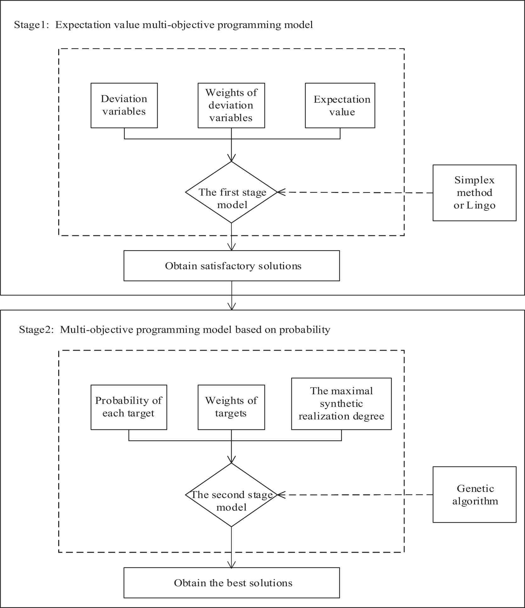
An overall process of two-stage random multi-objective programming model based on reliability (TS-MOPM).
The first stage model: Considering that the practical decision-making allows the target value to deviate within the limits. Our model will introduce the deviation variables to describe the difference between the objective function and the target value. Additionally, decision-makers may give different attentions (preferences) on the objectives, but these attentions still cannot reach obvious level difference. Therefore, our model will give different weights to different objectives. For the randomness in modeling, expectation value can be used to process random variables. Based on the above discussions the idea of model (3), the first stage model (expectation value multi-objective programming model) can be formulated as follows:
In model (5),
Model (5), a combination of model (2) and (3), has the following features: ① It can deal with uncertain programming problems by transformation; ② It can be solved directly by simplex method or lingo and has better solvability; ③ The existence of solution can be guaranteed. The fact that the target value allows some deviations demonstrates that a satisfactory solution can be obtained. However, model (5) still has some shortcomings: ① When the decision-making objectives have different dimensions, it is very difficult to give the reasonable explanation for the decision-making results; ② Model (5) only considers the expectation value of random variables, but missing the influence of variance. When the variables present great randomness, model (5) cannot guarantee the reliability of the results.
The second stage model: Under the framework of model (5), these expressions on real decision-making objectives, such as “Profits should not be less than a million yuan; Equipment occupy time should be b hours as much as possible; The raw material consumption should not be more than c kilogram as possible,” are the most common. Obviously, they have fuzziness and can be described as fuzzy events. For this case, it is necessary to deal with randomness and fuzziness simultaneously for solution. Probability theories are often used to deal with randomness. For instance, some scholars discussed the probability calculation method of fuzzy events with the aids of fuzzy set theories [33]. Zadeh [34] firstly proposed a probability calculation model of numerical fuzzy events of probability space with membership degree as the action coefficients. This method has good interpretability, but it cannot realize the probability calculation of algebraic operations of fuzzy events. Under the background of cognition inconsistency, Yager [35,36] proposed a fuzzy probability description strategy of fuzzy events, and gave two kinds computation methods based on cut sets. Based on the decomposition theorem of fuzzy sets and the probability of every cut set, Chen et al. [37] gave a probability calculation method of fuzzy events by using integral as a synthesis operator. Considering that decision-makers would show fuzzy preferences and each membership state would have nonlinear effect on the decision process, Li et al. [38] introduced the level effect function and further established an effect probability calculation method of fuzzy events.
For the fuzzy target value
In model (6), the importance weights of the targets value satisfy
Obviously, model (6) can make up for the deficiencies of model (5) to a certain extent, which can be stated as follows: ① Model (6) is a dimensionless model. It can better respond the uninterpretability of decision-making results caused by different target dimensions. ② Model (6) has good structural characteristics. Probability, a descriptive form of decision-making objectives, can directly reflect the realization degree of the target. Additionally, taking the synthetic realization degree of the first stage objective as a constraint, model (6) can not only reduce the range of solution, but also deduce whether there exists a solution with even higher reliability. ③ Model (6) has good interpretability. It can help decision-makers get the synthetic realization degree of the results under different conditions and the realization degree of each objective, which is very useful in explaining the implications of decision-making results.
Remark 1.
Model (6) aims at maximizing the synthetic realization degree of all the targets, without considering the realization degree of each single target. In particular, the constraints
TS-MOPM based on reliability improves expectation value model (3) and chance-constrained model (4) to a certain extent. It guarantees the existence of decision-making results, also considers the reliability at the same time. Therefore, TS-MOPM has better theoretical and instructive significance for decision-making problems under random environments.
4. SOLUTION STRATEGY FOR TS-MOPM
This section will discuss the probability calculation method of fuzzy event for several common distributions, and give the specific solution procedures of TS-MOPM.
In the following, we assume that
Let
Let
For
If A satisfies: ①
4.1. Probability Calculation of Fuzzy Events
This paper will use probability calculation model of [37], which is a special case of [38] for level effect function
Definition 1.
[37] Let
If we take the decision-making objective as fuzzy events, then the fuzziness of the target value can be described as fuzzy numbers, the most used fuzzy information description tool is triangular fuzzy number. Combining triangular fuzzy number, Eq. (7) with common distributions, for any continuous random variable X on probability space
In Eq. (8),
Theorem 1.
Let X be continuous random variables on
Proof:
According to Eq. (8) and
Combined with several common distributions, we have the following calculation formula based on Eq. (8) and Theorem 1.
Theorem 2.
Let X be continuous random variables on
If X obeys uniform distribution
If X obeys exponential distribution
If X obeys standard normal distribution
If X obeys normal distribution
Remark 2.
In practical decision-making, the results changing within a certain range of the target value are acceptable. However, the satisfaction degree will decrease with the deviation from the target value increasing. Therefore, this paper introduces the deviation parameter
X1 is not more than V1 as possible, then
X2 is not less than V2 as possible, then
X3 is equal to V3 as possible, then
Here,
Remark 3.
If we set
The above discussions can provide effective probability calculation of fuzzy events to a certain extent.
4.2. Solution Procedures of Solving TS-MOPM
Based on the probability calculation of fuzzy events proposed above, we will provide the complete solution procedures for solving TS-MOPM as follows:
[Begin]
Step 1 Obtain the satisfactory solutions of the first stage model (5)
Step 1.1 Set appropriate positive and negative deviation variables
Step 1.2 Initialize the expectation value
Step 1.3 Adopt simplex method or lingo software to obtain the satisfactory solutions
Step 2 Compute the probability of each target of model (5)
Step 2.1 Set deviation degree
Step 2.2 Compute the probability
Step 3 Set the weights
Step 4 Obtain the decision results of the second stage model (6) using Genetic algorithm
Step 4.1 Construct the population size
Step 4.2 Compute the fitness value
Step 4.3 Set crossover probability
Step 4.4 After
[End]
5. THE APPLICATION ANALYSIS OF TS-MOPM
5.1. Case Study
In this section, we will analyze the characteristics and test the effectiveness of TS-MOPM through a real case of multi-objective programming.
Case description: A pharmaceutical factory wants to produce two kinds of granular drugs M and N by using one raw material. According to previous statistics, the time required to produce 1 ton of M and N is
Set
In the following, we will give the solution of model (11) by TS-MOPM.
I The first stage model. Because equipment occupancy time X1, raw materials X2, and total profit X3 are random variables obeying normal distribution, they can be quantified through expectation values, i.e.,
Use lingo to solve (12), the solution results are stated as Table 1 in the following:
| Parameter | x1 | x2 | |||||
|---|---|---|---|---|---|---|---|
| w1 = 0.8 | |||||||
| Case 1 | w2 = 0.1 | 22.5 | 18.75 | 0 | 0 | 11.25 | 0 |
| w3 = 0.1 | |||||||
| w1 = 0.1 | |||||||
| Case 2 | w2 = 0.8 | 24.4565 | 16.3044 | 5.8696 | 0 | 4.8913 | 0 |
| w3 = 0.1 | |||||||
| w1 = 0.1 | |||||||
| Case 3 | w2 = 0.1 | 24.4565 | 16.3044 | 5.8696 | 0 | 4.8913 | 0 |
| w3 = 0.8 | |||||||
| w1 = 0.4 | |||||||
| Case 4 | w2 = 0.4 | 24.4565 | 16.3044 | 5.8696 | 0 | 4.8913 | 0 |
| w3 = 0.2 | |||||||
| w1 = 0.4 | |||||||
| Case 5 | w2 = 0.2 | 22.5 | 18.75 | 0 | 0 | 11.25 | 0 |
| w3 = 0.4 | |||||||
| w1 = 0.2 | |||||||
| Case 6 | w2 = 0.4 | 24.4565 | 16.3044 | 5.8696 | 0 | 4.8913 | 0 |
| w3 = 0.4 | |||||||
| w1 = 1/3 | |||||||
| Case 7 | w2 = 1/3 | 24.4565 | 16.3044 | 5.8696 | 0 | 4.8913 | 0 |
| w3 = 1/3 | |||||||
Results obtained from the first stage.
Table 1 presents all the satisfactory solutions with different objective weights. We can see that, the deviations of total profits are 0 as the weights change. It is because that “the magnitude of profit is larger than the other two targets values.” This fact leads to no significant changes of the solution results. Moreover, the results have the following two shortcomings: ① Taking the minimum absolute deviation as the objective, the reliability of the decision-making results cannot be demonstrated, which is an important index evaluating the decision-making quality; ② The required decision-making objectives have different dimensions. Therefore, it is difficult to explain the practical meaning of the decision-making results explicitly.
II The second stage model. According to Theorem 1 and Remark 2, the satisfactory state value of the equipment occupy time can be expressed as
According to Theorem 2, it is difficult to determine the numerical computation of
We use GA to obtain various results under different decision-making preference listed in Table 2. Particularly, GA works with binary-encoded strings with length 20. Set the size of population as 80, crossover probability as
| Parameters | x1 | x2 | ||||||
|---|---|---|---|---|---|---|---|---|
| w1 = 0.8 | ||||||||
| Case 1 | w2 = 0.1 | 0.6266 | 24.7067 | 17.6442 | 0.6593 | 0.1737 | 0.9917 | 0.6440 |
| w3 = 0.1 | ||||||||
| w1 = 0.1 | ||||||||
| Case 2 | w2 = 0.8 | 0.5246 | 24.4565 | 16.3044 | 0.4188 | 0.5057 | 0.7816 | 0.5246 |
| w3 = 0.1 | ||||||||
| w1 = 0.1 | ||||||||
| Case 3 | w2 = 0.1 | 0.7171 | 24.5601 | 17.8299 | 0.6559 | 0.1587 | 0.9918 | 0.8749 |
| w3 = 0.8 | ||||||||
| w1 = 0.4 | ||||||||
| Case 4 | w2 = 0.4 | 0.5261 | 24.6090 | 17.0127 | 0.6037 | 0.3062 | 0.9516 | 0.5543 |
| w3 = 0.2 | ||||||||
| w1 = 0.4 | ||||||||
| Case 5 | w2 = 0.2 | 0.6320 | 24.6090 | 17.4770 | 0.6551 | 0.2120 | 0.9827 | 0.6975 |
| w3 = 0.4 | ||||||||
| w1 = 0.2 | ||||||||
| Case 6 | w2 = 0.4 | 0.5987 | 24.8534 | 16.8915 | 0.6042 | 0.3006 | 0.9669 | 0.6278 |
| w3 = 0.4 | ||||||||
| w1 = 1/3 | ||||||||
| Case 7 | w2 = 1/3 | 0.5687 | 25.0 | 16.8456 | 0.6089 | 0.2914 | 0.9755 | 0.6253 |
| w3 = 1/3 | ||||||||
Results obtained from the second stage.
From Table 2, we know that, ① Compared with Table 1, the decision-making results of Table 2 are more sensitive to the change of weight, which shows that the attention degree of each objective will directly affect the decision-making results; ② Under different decision-making states, the synthetic realization degree of the objectives in the second stage is higher than that in the first stage. Occasionally, the synthetic realization degree is the same as case 2. All these indicate that TS-MOPM has higher reliability than expectation value model in decision-making results. So TS-MOPM has important reference value and instructive guide; ③ TS-MOPM has good interpretability. Both the synthetic reliability of decision-making results with different preferences and the realization degree of each objective can be directly obtained, which is beneficial for the explanation of the implications of the results under different states.
5.2. Other Applications
Two stage multi-objective programming techniques under random environment have been widely applied to handle many real decision problems.
Transportation network design. In recent years, as the travel demands rise continuously, severe traffic congestion and transportation delays are often incurred. Optimize transportation network is becoming urgent problems in urban transportation planning. In regard to designing traffic network, transportation cost is of vital importance in the overall transportation process. Additionally, with the development of resource-efficient and sustainable cities, high efficiency and environmental protection are also the main concerns strived for in decision-making process. Therefore, transportation network design can be posed as a multi-objective programming problem. Transportation cost, transportation time and emissions are three critical aspects that management must minimize to optimize a network. Nevertheless, the randomness of transportation requirements cause the uncertainty of three indexes in an actual integrated freight system. In most cases, three objectives are not of equal importance. In a word, the mentioned problem can be solved through establishing a two stage multi-objective programming model.
Supplier selection and management. Supply chain management requires harmonizing the business processes among the members, i.e., suppliers, producers, and distributors. In most industries, the cost of raw material constitutes a large portion of products price. Therefore, to reduce the production cost of a product, it is increasingly important to select appropriate suppliers which can directly influence the efficiency of the business [7]. Additionally, the ever changing complexity of competitive environment makes cost minimization not the only objective, other factors such as the quality of raw materials and on-time delivery are of great significance. Nevertheless, all the indexes “cost minimization, good quality and on-time delivery” have uncertainty. Coupled with the variability of business environment, the supplier selection problem can be investigated through two stage multi-objective programming model.
6. CONCLUSIONS
For random numerical multi-objective decision-making problems, this paper extends the previous researches and establishes TS-MOPM by taking fuzzy decision-making objective as fuzzy events. TS-MOPM has the following advantages:
First, TS-MOPM uses probability to describe all the decision-making objectives. It can eliminate the dimensional influence on the explanation of decision-making results, and make up for the deficiencies of priority factor model to some extent. Moreover, the probability calculation of fuzzy events has generality. Therefore, TS-MOPM has general applications.
Second, TS-MOPM tells the decision-makers the realization degree of decision-making results intuitively. Even if the randomness is even greater, the decision-making results can also be guaranteed. It makes up for the deficiencies of expectation value model.
Third, TS-MOPM has better operability and solvability. It can avoid high computation complexity due to too many decision-making objectives and no solution due to inappropriate confidence level for chance- constrained programming model.
The probability calculation involved in TS-MOPM is a key issue in its application. Although Section 4 gives several methods of some special fuzzy events, these work cannot fairly meet decision-making needs in complex random environment. Thus, further work is needed to construct probability calculation platform based on stochastic simulation and decision-making system based on probability.
CONFLICT OF INTEREST
We declare that we do not have any commercial or associative interest that represents a conflict of interest in connection with the work.
AUTHORS' CONTRIBUTIONS
Chenxia Jin: Conceptualization, Writing - review & editing. Fachao Li: Visualization. Kaixin Feng: Writing - original draft. Yunfeng Gup: Software.
ACKNOWLEDGMENTS
This work is supported by the National Natural Science Foundation of China (71771078, 71371064) and Graduate research and innovation projects of Hebei Province (CXZZBS2020076).
REFERENCES
Cite this article
TY  - JOUR
AU  - Chenxia Jin
AU  - Fachao Li
AU  - Kaixin Feng
AU  - Yunfeng Guo
PY  - 2020
DA  - 2020/04/27
TI  - A Two-Stage Multi-objective Programming Model to Improve the Reliability of Solution
JO  - International Journal of Computational Intelligence Systems
SP  - 433
EP  - 443
VL  - 13
IS  - 1
SN  - 1875-6883
UR  - https://doi.org/10.2991/ijcis.d.200410.001
DO  - 10.2991/ijcis.d.200410.001
ID  - Jin2020
ER  -