
Sparse Least Squares Support Vector Machine With Adaptive Kernel Parameters
- DOI
- 10.2991/ijcis.d.200205.001How to use a DOI?
- Keywords
- Least squares support vector machine; Sparse representation; Dictionary learning; Kernel parameter optimization
- Abstract
In this paper, we propose an efficient Least Squares Support Vector Machine (LS-SVM) training algorithm, which incorporates sparse representation and dictionary learning. First, we formalize the LS-SVM training as a sparse representation process. Second, kernel parameters are adjusted by optimizing their average coherence. As such, the proposed algorithm addresses the training problem via generating the sparse solution and optimizing kernel parameters simultaneously. Experimental results demonstrate that the proposed algorithm is capable of achieving competitive performance compared to state-of-the-art approaches.
- Copyright
- © 2020 The Authors. Published by Atlantis Press SARL.
- Open Access
- This is an open access article distributed under the CC BY-NC 4.0 license (http://creativecommons.org/licenses/by-nc/4.0/).
1. INTRODUCTION
Least Squares Support Vector Machine (LS-SVM) algorithm has received a great deal of attention over the last two decades. By mapping the input data into a high-dimension feature space, LS-SVM algorithm is able to learn complex non-linear relationship from training samples. Due to this advanced learning capability, relevant application has spanned several disciplines, such as pattern recognition, decision making, and statistical modeling. The wide applicability also has motivated growing interest in developing efficient LS-SVM training algorithms with fast convergence and good generalization ability.
One major drawback with conventional LS-SVM based algorithms is the solution's sparsity, in which a great number of support vectors (SVs) are required in the resultant model [1–3]. The SVs are typically a portion of training samples, used to determine the decision boundary. However, too many SVs might have a negative impact on the generalization ability of the trained model, not to mention larger computational cost. In addition, computational complexity scales with the increasing number of SVs. To address the problem associated with large number SVs, a variety of sparsity-enhanced approaches have been applied, where significant SVs are determined and selected to form the decision boundary. For instance, Suykens et al. first proposed removing training samples that have the smallest absolute support values [2]. However, this method might eliminate training samples near the decision boundary, which has a negative influence on the training performance. An improved method was proposed in [3], in which a reduced training set is only comprised of samples near the decision boundary. Another sparsity-enhanced method was proposed in [4], in which least-important SVs are removed through regularization (i.e., Nyström approximation) to accelerate the training process. In [5], SVs were eliminated using single and multi-objective evolutionary computation approaches, without affecting the classifier accuracy and even improving it.
Another problem of traditional LS-SVM training is to determine the suitable kernel parameters, that are associated with the employed kernel function. For instance, in the Gaussian Radial Basis Function (RBF), the kernel parameter is the smoothing parameter (also known as the kernel size or bandwidth). Then, before any training process, kernel parameters will need to be pre-determined and fixed. However, the parameter setting is purely data-driven, as the optimal value varies case-by-case. Additionally, the resultant performance using different settings of kernel parameters can greatly differ from each other. As there is not a rule of thumb to determine the optimal kernel parameters, trial-and-error or cross-validation experiments are often required, which can be very time-consuming.
In our previous work [6], we have presented one sparse training algorithm, in which the LS-SVM training is reformulated as a sparse representation process. As such, the training is accomplished by iteratively finding important SVs that minimize the training error. In this paper, additionally, we introduce a dictionary-learning inspired technique to further optimize the kernel-based training. The aim is to enhance the model sparsity without compromising the training performance. Toward this end, a kernel matrix is firstly established using training samples, and later formulated as the dictionary. Then the dictionary-learning algorithm is employed to explore the optimal parameter via minimizing the average coherence of this kernel matrix (i.e., dictionary). When the sparse representation and dictionary learning techniques are combined, the proposed algorithm is able to perform model training, SVs selection, and kernel parameters optimization simultaneously.
The remainder of the paper is organized as follows. Section 2 gives a brief introduction about kernel-based learning algorithms (such as Support Vector Machine [SVM] and LS-SVM). Section 3 provides the basic concept about sparse representation and dictionary learning, respectively. Section 4 presents the proposed sparsity-enhanced training approach, including applying the sparse representation technique to select important SVs and optimizing kernel parameters based on the dictionary-learning concept. Section 5 compares the proposed algorithm with conventional training methods using several benchmark problems. Section 6 presents concluding remarks.
2. KERNEL-BASED LEARNING ALGORITHMS
In this section, we first introduce the general formulation of the kernel-based learning algorithms. Then the SVMs and LS-SVMs will be discussed as two of the most popular kernel learning techniques, respectively.
Recent years have witnessed the rapid development of the kernel-based learning methods, and their wide applications in several applications, such as classification, pattern recognition, and many more. Generally speaking, the fundamental strategy of kernel-based learning is to map raw data from the original space into a Hilbert space with higher dimension, using some kernel functions. The advantage is that in the Hilbert space, more effective separation hyperplanes are expected to exist compared to the original space.
The most-used kernel functions are liner, polynomial, and RBF kernels. Among various kernels, RBF kernel is very popular and usually used as a default choice due to its desirable smoothness and numeric stability. Therefore, in this paper the RBF function is employed which is expressed as
Before training, however, we need to pre-determine the value of the kernel size or
2.1. Support Vector Machines
As one of the most popular kernel-based approaches, the SVM algorithm has been demonstrated to perform well in various practical applications. The SVM model is fundamentally formulated to address two-class classification problems. The decision boundary is constructed by finding a hyperplane that achieves the maximum separation between two classes. Suppose that we have a training set consisting of
Note that there exist more than one hyperplanes that can separate the two classes; however, only one of them, termed optimal separating hyperplane, can maximize the margins between the two classes. Consequently, the SVM training is to find
The parameter optimization in Eq. (3) is built on the assumption of linear separability of the training data. However, if the problem is not linearly separated in the original space, an SVM classifier with a linear decision boundary will have a poor generalization ability. To improve the classification accuracy, the data samples are usually projected from the input space to a higher-dimensional space via a mapping function
2.2. Least Squares Support Vector Machines
LS-SVMs have been developed to achieve more affordable and faster training. As a variant of SVM, in the LS-SVM model, the inequality constraints in Eq. (3) are replaced with equality constraints, and the unknown parameters are then obtained by solving the following problem:
Furthermore, the above conditions lead to a linear system of equations after eliminating
With the application of Mercer's theorem, there is no need to compute explicitly the mapping
The traditional training algorithm for LS-SVM is to use the conjugate gradient (CG). One common problem comes from the large number of SVs required in training, which may influence the generalization capability. Therefore, several optimization methods have been suggested to improve the sparsity of the LS-SVM model (i.e., minimizing the number of required SVs). Some of those early studies include [1–3] (mentioned in Section 1).
More recent studies include CLS-SVM [6], SSS [10], and SLQ [11]. For instance, in [6], the CLS-SVM algorithm is the first attempt to train the LS-SVM using the concept of the sparse representation. Additionally, the SSS algorithm in [10] conducts the training process based on a graph Laplacian matrix
3. SPARSE REPRESENTATION AND DICTIONARY LEARNING
Over the past decade, signal sparse representations have received extensive research interests across several communities, including image processing [12], machine learning [13], and simulation [14]. The fundamental concept underlying sparse representation indicates that a signal can be approximated by a linear combination of a few elementary signals. Alternatively, few elements are capable of representing the majority information conveyed by the target signal.
3.1. Single Measurement Vector Model
The single measurement vector (SMV) model is one typical model for sparse representation. The aim of the SMV model is to recover a sparse signal
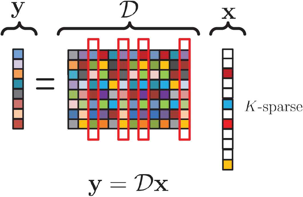
The SMV model aims to minimize a vector sparsity. In the sparse signal
To measure the sparsity
A variety of algorithms have been developed to solve the SMV model. For instance, the Orthogonal Matching Pursuit (OMP) algorithm is a popular algorithm that offers a good sparse solution [15]. During the iterative process, it will first measure the similarity between the residual error and the dictionary columns, and then select the column that minimizes the error most. In this paper, we will utilize OMP in our experiments to calculate the sparse solution.
3.2. Dictionary Learning
Solving the SMV model, however, relies heavily on the employed dictionary structure, or the degree of fitting between the data and the dictionary [16,17]. A randomly initialized dictionary
Definition 1.
The mutual coherence
In general, a dictionary consisting of more similar columns has a higher
4. PROPOSED SPARSE LS-SVM
In this section, we present a sparsity-enhanced algorithm, termed Adaptive-Kernel based Sparse Learning (AKSL), to address two main issues associated with the LS-SVM training, i.e., solution sparsity and kernel parameter optimization. The main difference between AKSL and existing LS-SVM technique is that the proposed method is capable of training the model using less SVs and optimizing the kernel parameter simultaneously.
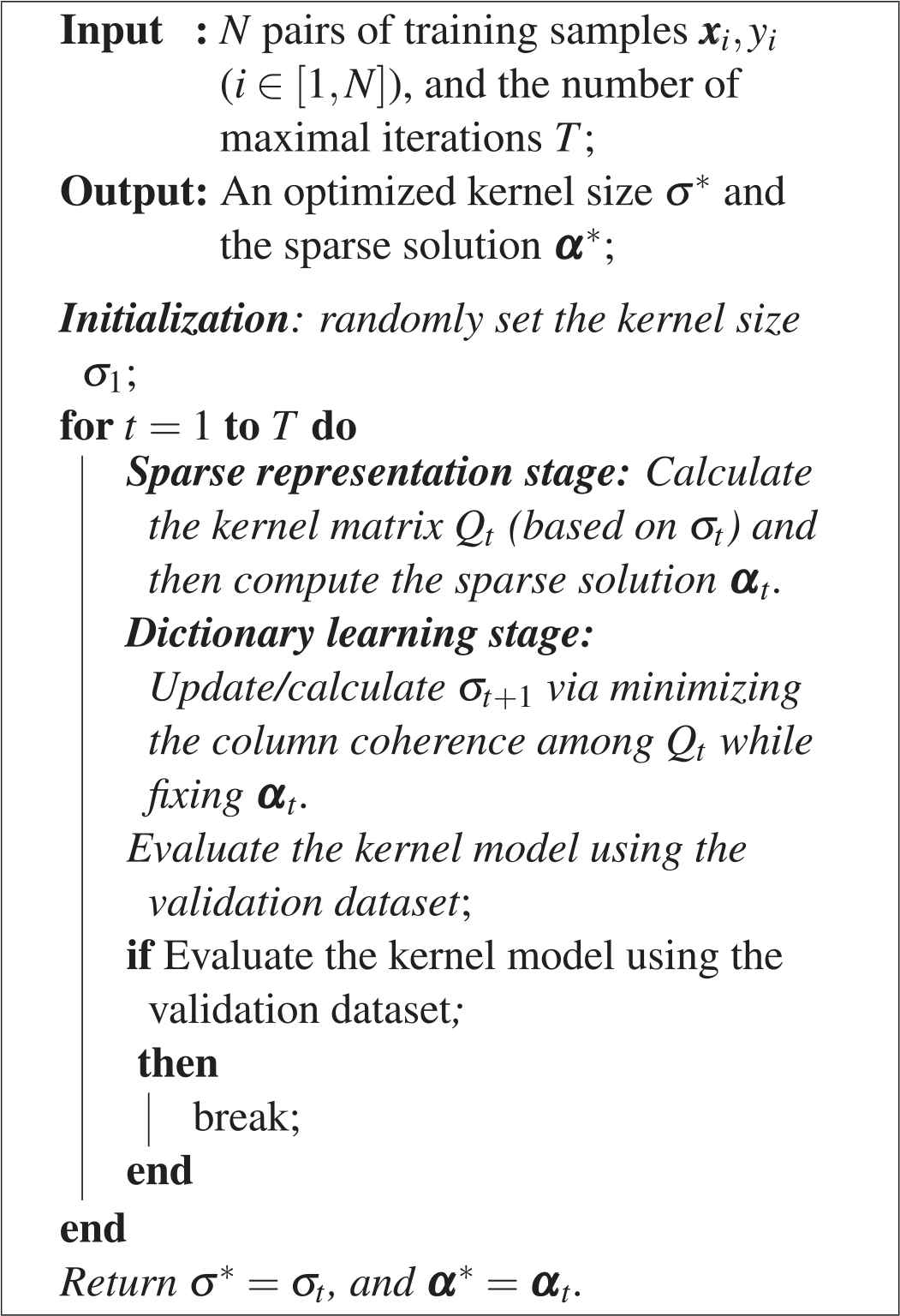
Overall, the proposed AKSL algorithm consists of two stages: sparse representation and dictionary learning. See Algorithm 1 for the general diagram of the proposed AKSL algorithm. In the sparse representation stage, the goal is to conduct kernel-based training via forming a sparse solution. Additionally, the stage of dictionary learning is characterized by adjusting the kernel parameter while fixing the sparse solution. Toward this end, in Section 4.1, we formulate the LS-SVM training as a sparse representation process. In Section 4.2, we introduce a heuristic approach (based on the dictionary learning) to optimize kernel parameters.
4.1. Sparsity-Enhanced Training
Suppose that we have a training set consisting of
Algorithm 1: The proposed sparsity-enhanced algorithm (AKSL) for the LS-SVM training.
To simply the process, we skip the bias term
Nevertheless, the computation of
Note that setting a particular element of
Algorithms that applied to solve the SMV model can be accordingly employed for Eq. (12). Herein, we use the OMP algorithm [15]. The reason is two-fold: (i) the OMP algorithm has been proven to be effective for solving the SMV model in numerous case studies; and (ii) more importantly, via OMP we can control the sparsity or number of non-zero elements in the solution
4.2. Kernel Parameter Optimization Using Dictionary Learning
During the sparse representation stage, the proposed algorithm generates a compact model by selecting most significant elements from
Toward this end, we introduce a two-step methodology to systematically conduct the
Second, we further like to minimize the mutual coherence of the dictionary (i.e.,
However,
Definition 2.
For a dictionary
Note that the proposed
To minimize
On the other hand, to compute
Immediately, we have
Overall, the
The Lagrangian function of Eq. (18) can be written as:
For simplicity, let
On the other hand, from the definition of RBF kernel function in Eq. (1), it is easy to know
Note that
5. EXPERIMENTAL RESULTS
This section presents the experimental results and comparisons of the proposed algorithm with conventional training techniques. The employed classification data sets and the evaluation of the training algorithms are presented in Section 5.1. The performance of the proposed algorithm is then evaluated in Section 5.2. The comparison results with conventional training algorithms are presented in Section 5.3.
5.1. Experimental Methods
Several classification problems are chosen from UCI repository [20] for the experimental evaluation (see Table 1). These problems are selected so as to ensure a good coverage of sample sizes, output dimensions (multiple and binary), variable types (discrete and continuous), and attribute numbers.
| Data Set | #.Features | #.Size | Classes |
|---|---|---|---|
| Leaf | 16 | 340 | Binary |
| Online (News Popularity) | 60 | 39797 | Binary |
| Adult | 14 | 32562 | Binary |
| Badges | 26 | 294 | Binary |
| Breastcancer | 10 | 699 | Binary |
| Ionosphere | 34 | 351 | Binary |
| Contraceptive | 9 | 1473 | Multiple |
| Dermatology | 34 | 366 | Multiple |
| Glass | 10 | 214 | Multiple |
| Wine | 13 | 178 | Multiple |
Employed classification datasets from UCI.
To measure the performance of the proposed algorithm, we applied the 4-fold cross validation and randomly partitioned one entire data into three independent sets: a training set, a validation set, and a testing set. The size of the training, validation and testing sets in all cases is 50%, 25%, and 25%, respectively. Additionally, training samples will firstly be standardized to zero mean and unit variance.
The solution sparsity or the model structure is measured as follows:
Additionally, the proposed training algorithm is terminated if the error on the validation set increases for a few successive iterations (empirically, the value is set as three). This is a common strategy for terminating training in other existing work [21]. The penalty term of
5.2. Performance Analysis of AKSL
In this section, we first investigate the effect of the solution sparsity on the generalization ability. Second, we test the performance of the proposed method with the optimized kernel size.
5.2.1. Support vectors
The number of SVs is critical to the performance of the AKSL algorithm. For instance, too many SVs might have a negative impact on the generalization ability, not to mention larger computational cost. Therefore, in this section we analyze how the number of SVs impacts the performance of AKSL. The remaining model structure is set to
Table 2 shows the performance of the proposed algorithm with respect to the remaining model structure. As can be observed, the proposed method achieves a better classification accuracy on the training sets with increasing number of SVs. The performance on the training sets is 96.43%, 98.43%, 99.39%, 99.83%, and 99.96% for
| DataSets | k | 20% | 30% | 50% | 70% | 100% |
|---|---|---|---|---|---|---|
| Training | 96.81% | 98.95% | 99.89% | 100.00% | 100.00% | |
| Leaf | Test | 68.21% | 68.57% | 71.96% | 68.95% | 70.36% |
| Training | 92.09% | 97.52% | 100.00% | 100.00% | 100.00% | |
| Online | Test | 70.02% | 69.46% | 67.81% | 69.72% | 67.96% |
| Training | 97.67% | 98.77% | 99.58% | 99.83% | 100.00% | |
| Adult | Test | 81.80% | 82.25% | 84.94% | 82.73% | 86.68% |
| Training | 93.69% | 100.00% | 100.00% | 100.00% | 100.00% | |
| Badge | Test | 69.87% | 73.16% | 73.29% | 80.92% | 78.03% |
| Training | 100.00% | 100.00% | 100.00% | 100.00% | 100.00% | |
| Breastcancer | Test | 98.87% | 98.85% | 98.81% | 98.35% | 99.28% |
| Training | 88.06% | 91.98% | 95.63% | 98.44% | 99.57% | |
| Contraceptive | Test | 80.51% | 83.18% | 89.82% | 79.37% | 74.10% |
| Training | 99.95% | 99.99% | 100.00% | 100.00% | 100.00% | |
| Dermatology | Test | 96.12% | 96.56% | 95.16% | 93.08% | 95.97% |
| Training | 96.02% | 97.29% | 98.82% | 99.99% | 100.00% | |
| Glass | Test | 78.33% | 79.31% | 71.43% | 72.22% | 77.09% |
| Training | 99.96% | 99.84% | 100.00% | 100.00% | 100.00% | |
| Ionosphere | Test | 96.56% | 92.40% | 97.33% | 90.32% | 97.39% |
| Training | 100.00% | 100.00% | 100.00% | 100.00% | 100.00% | |
| Wine | Test | 91.67% | 100.00% | 100.00% | 100.00% | 96.25% |
| Training | 96.43% | 98.43% | 99.39% | 99.83% | 99.96% | |
| Average | Test | 76.20% | 77.37% | 79.06% | 78.52% | 78.31% |
Note. AKSL = adaptive-Kernel based Sparse Learning.
Summary of the classification accuracy (%) from the proposed AKSL method. Various numbers of selected support vectors are considered.
5.2.2. Kernel size optimization
The adaptive kernel-size technique is considered in the proposed algorithm, which is used to obtain a suitable value for the kernel size (i.e.,
The evolutionary curve related to the average mutual coherence (
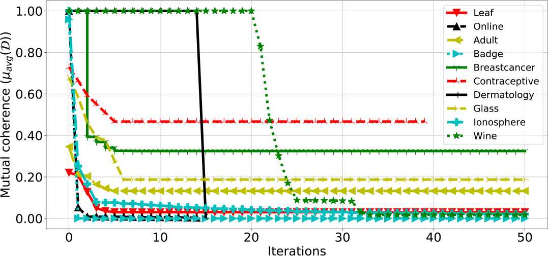
Related average mutual coherence
The next experiment explores the effect of the adaptive
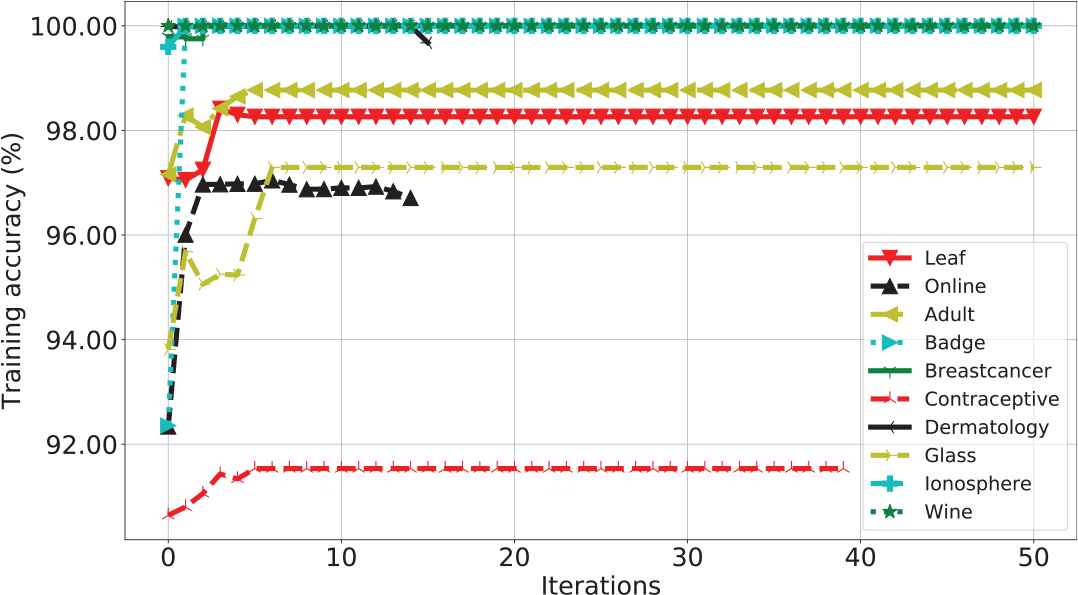
Evolutionary curve of the training accuracy (%) from the proposed algorithm for employed datasets.
5.3. Comparison with Other Training Algorithms
In this section, the proposed AKSL algorithm is compared with five conventional sparse training algorithms, namely CLS-SVM [6], SSS [10], SLQ [11], CCS [22], and VSS [9]. We have briefly introduced the algorithm of CLS-SVM, SSS, and SLQ in Section 2. For CCS, it has been proposed to enhance the traditional LS-SVM by minimizing the number of SVs. The major contribution is that CCS adopts a Singular Value Decomposition (SVD) to form a measurement matrix
Note that all algorithms of CLS-SVM, SSS, SLQ, and CCS are aiming for reducing the number of SVs and maximizing the solution sparsity. To make a fair comparison, for these sparsity-based algorithms, we apply the same least number of SVs (i.e., set
On the other hand, the VSS method presented in [9] is to solve a least-mean-square based problem with adaptive kernel-sizes. The major difference of VSS, compared to others, is that VSS does not consider the solution sparsity, but only optimizes the kernel size.
Figures 4 and 5 presents the average training and test accuracy obtained from different methods, respectively, while the accuracy standard deviation is also provided. Compared to conventional training algorithms, the proposed AKSL algorithm achieves a significant improvement in terms of classification accuracy. For instance, using the same number of SVs (
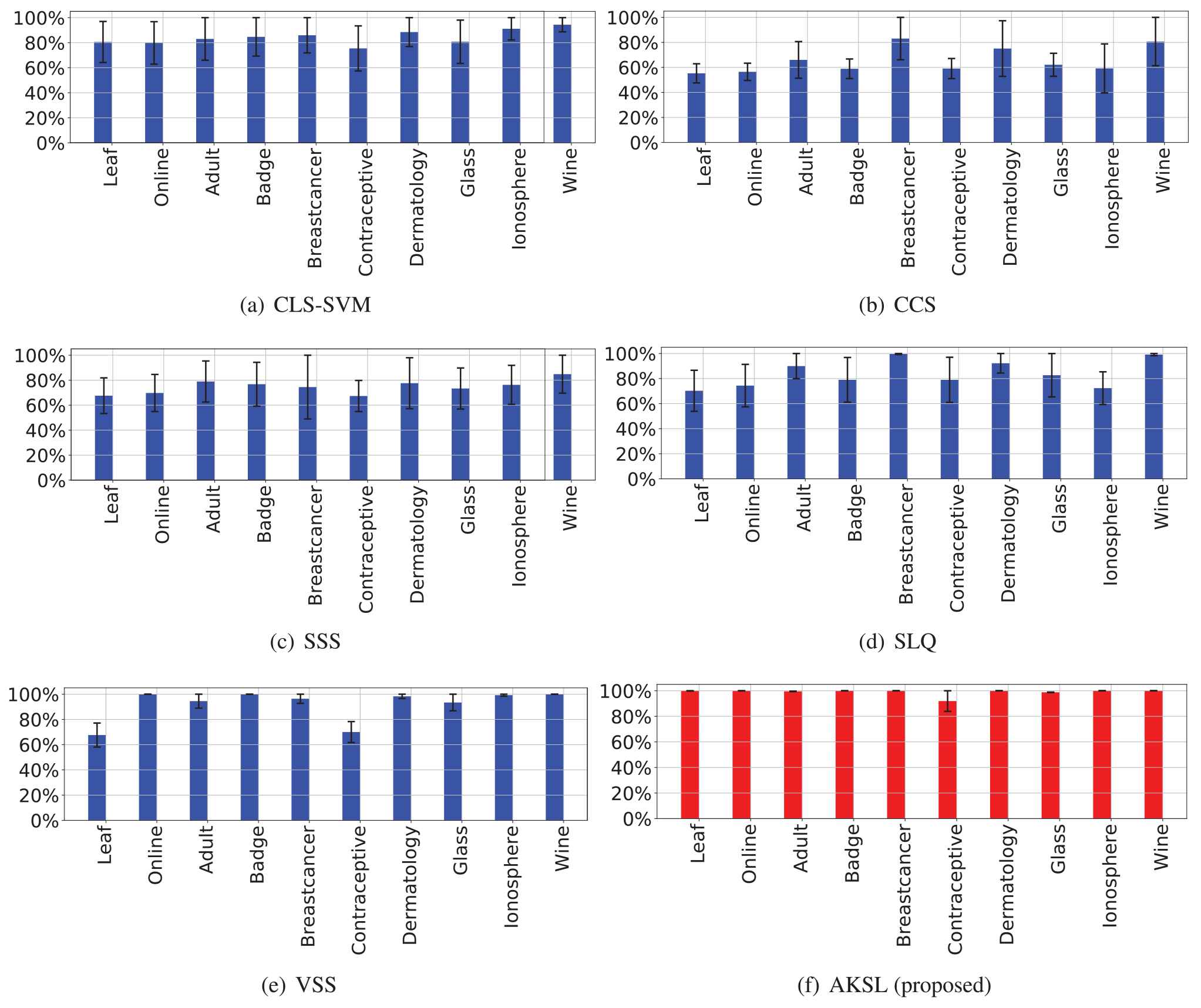
Average training accuracy obtained from different algorithms for the classification tasks, while black lines represent the confidence intervals at the 95% level.
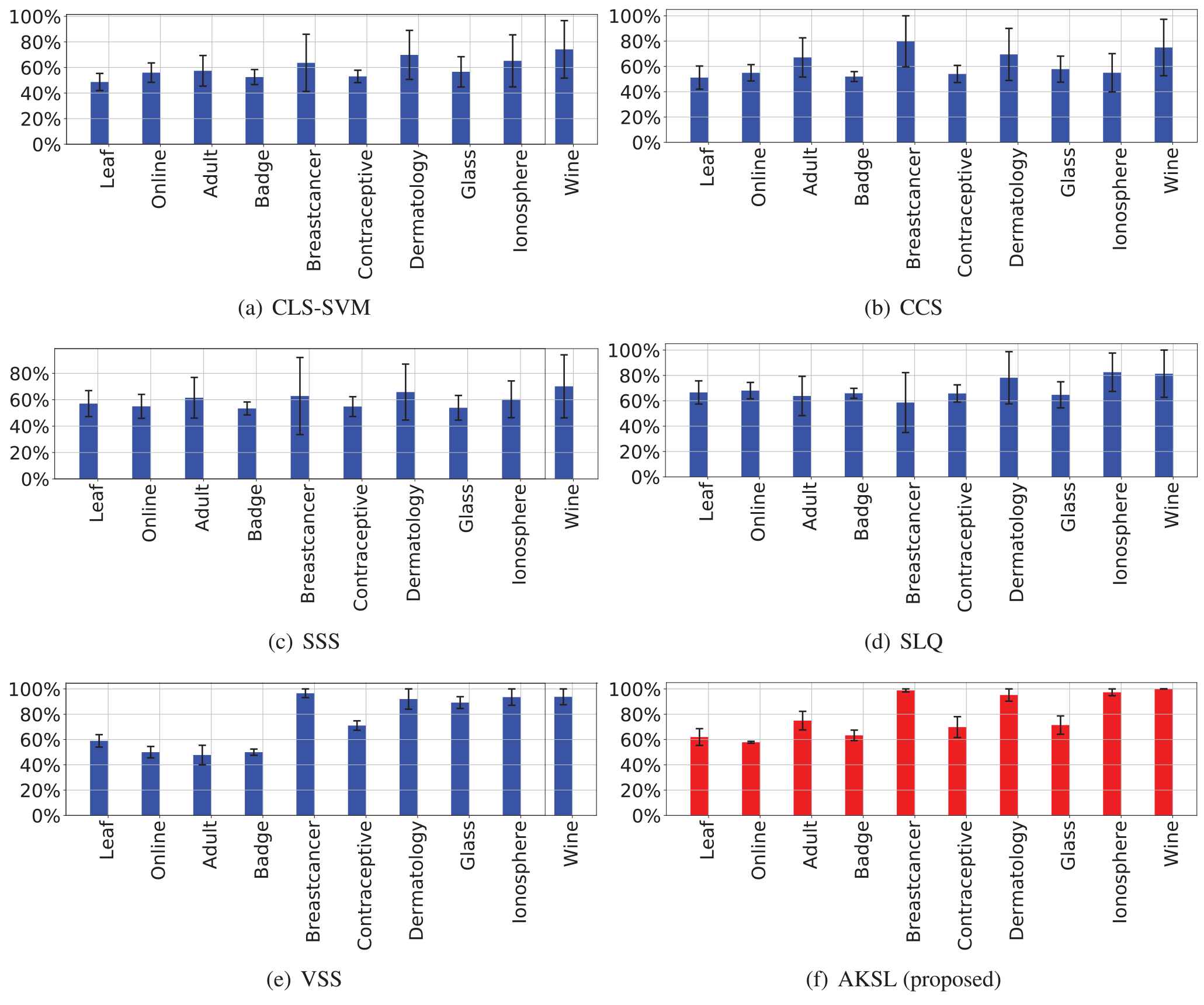
Average test accuracy obtained from different algorithms for the classification tasks; again, the error bars are associated with the confidence intervals at the 95% level.
We then investigated the computational complexity of all training algorithms. Figure 6 presents the average training time. The proposed algorithm spends 44.68 seconds on average to solve those benchmark problems, which is much better than the training time of SSS (270.70s), SLQ (266.72s), and VSS (62.58s) methods. However, the required time for CLS-SVM (7.59s) and CCS (17.89s) is shorter than the proposed algorithm. The reason could be both CLS-SVM and CCS algorithm do not consider to optimize the kernel size, but only concerns about the sparse solution. Nevertheless, the performance from AKSL is much better than that of CLS-SVM and CCS in terms of the training/testing accuracy, which compensates for its long computational time.
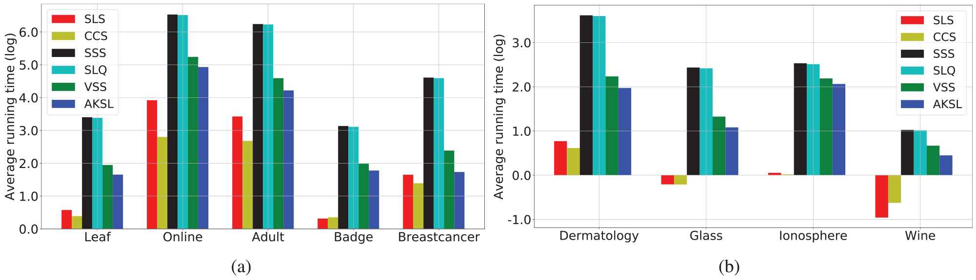
Average training time (log) obtained from different algorithms for the classification tasks.
In conclusion, it can be empirically confirmed that the proposed AKSL algorithm outperforms existing state-of-the-art approaches, in terms of solution sparsity (less SVs) and generalization ability. Again, starting from the empty solution, AKSL iteratively selects significant SVs that minimize the training error. This method can be regarded as a forward selection instead of backward elimination, therefore a fast convergence is expected. Furthermore, the proposed approach employs the dictionary-learning technique to optimize the kernel size, instead of traditional cross-validation methods. As a result, the AKSL algorithm achieves an affordable training time and satisfactory classification accuracy.
6. CONCLUSION
In this study, we have proposed an improved training method for LS-SVM, based on sparse signal representation and dictionary learning. The kernel matrix formed using training inputs is regarded as a dictionary in the sparse representation, consequently casting the training process to simply finding a sparse solution for the kernel classifier. The dictionary learning technique is also introduced to further optimize the kernel size during the training process. More precisely, the kernel size is optimized in the way that the average coherence of the kernel matrix is minimized. The main difference between AKSL and existing LS-SVM techniques is that the proposed method is capable of selecting important SVs, training the classification model, and optimizing the kernel size simultaneously. Several benchmark classification problems are chosen for the experimental evaluation. Results demonstrate that the proposed training method leads to competitive performance, in terms of the sparse model and satisfactory classification accuracy.
CONFLICT OF INTERESTS
The authors declare that they have no known competing financial interests or personal relationships that could have appeared to influence the work reported in this paper.
AUTHORS' CONTRIBUTIONS
Chaoyu Yang is responsible for the Conceptualization, Methodology, Software, Validation, Investigation, Visualization, and Writing of the original draft. Jie Yang and Jun Ma are responsible for the Software, Writing–Review and Editing, and Supervision of the original manuscript.
ACKNOWLEDGMENTS
This work was partially supported by the National Natural Science Foundation of China (Grant No. 61873004), and the Humanities and Social Sciences Foundation of Anhui Department of Education, China (Grant No. SK2017A0098).
Footnotes
Available from https://scikit-learn.org.
REFERENCES
Cite this article
TY  - JOUR
AU  - Chaoyu Yang
AU  - Jie Yang
AU  - Jun Ma
PY  - 2020
DA  - 2020/03/02
TI  - Sparse Least Squares Support Vector Machine With Adaptive Kernel Parameters
JO  - International Journal of Computational Intelligence Systems
SP  - 212
EP  - 222
VL  - 13
IS  - 1
SN  - 1875-6883
UR  - https://doi.org/10.2991/ijcis.d.200205.001
DO  - 10.2991/ijcis.d.200205.001
ID  - Yang2020
ER  -