
Optimisation of Group Consistency for Incomplete Uncertain Preference Relation
- DOI
- 10.2991/ijcis.d.200121.002How to use a DOI?
- Keywords
- Incomplete preference relation; Group decision making; Additive consistency; Uncertainty theory
- Abstract
An incomplete uncertain preference relation (UPR) is typical in group decision making (GDM) for decision makers (DMs) to express preference over alternatives because of the information interaction barrier between people and decision making environment. Completing missing values can guarantee individual consistency and consensus level effectively. The operation of traditional interval preference relations (IPRs) is based only on the end point transformation, which may cause interval discretisation and information distortion easily. To overcome these limitations, pairwise comparison of alternatives in an IPR is treated as an uncertain distribution function of the subjective preference of the DM which avoids discretisation operation and handles interval numbers collectively. A belief degree is used to maintain the original information as much as possible. It guarantees the extent how people believe the estimated value is close to the incomplete original value. An uncertain chance constrained programming model is proposed herein to estimate incomplete values based on a belief degree when the preference relation obeys a linear uncertain distribution. A distance measure is defined to compute the consistency index and consensus degree. Subsequently, an iterative algorithm is presented for GDM with linear UPRs, which adjusts inconsistent preference relations and uses an operator to aggregate all individual preference relations. Furthermore, it is proven that the operation of UPRs is an extension of that of traditional IPRs under a certain belief degree.
- Copyright
- © 2020 The Authors. Published by Atlantis Press SARL.
- Open Access
- This is an open access article distributed under the CC BY-NC 4.0 license (http://creativecommons.org/licenses/by-nc/4.0/).
1. INTRODUCTION
Interval preference relations (IPRs) have been widely used in uncertain group decision making (GDM) to represent decision makers’ (DMs’) preference over alternatives. When encountering complex or emergent situations, DMs cannot express their complete preference information on alternatives and often present an incomplete (sparse) form of judgment because of knowledge reserve, information mastery, environment impact, and so on. Incomplete IPRs can be managed by two approaches. One is filling in incomplete values based on consistency [1–6], and the other is ranking alternatives directly with known elements [7–9]. Although the latter preserves the true preferences of DMs, it cannot guarantee the consistency between individuals, thus resulting in the distortion of decision making. Based on consistency, the iterative algorithm [10–13] and the optimisation model [4,14–17] are two typical methods to complete missing values. Based on the iterative algorithm, although it is easy to change the original preference relations and the convergence speed is slow, the process is robust and the consistency is good. Furthermore, the optimisation model with missing parameter constraints can obtain the optimal solutions of incomplete values.
The consistency index is typically used for measuring the consistency level of an individual IPR; subsequently, an iterative algorithm is established to achieve an acceptable level of consistency, such as in an interval fuzzy preference relation (IFPR) [18,19], interval intuitionistic preference relation [20–22], linguistic preference relation [23,24], and hesitant fuzzy preference relation (FPR) [25,26]. The compatibility [27–32] is used similar to the consistency index. To ensure the efficiency and consensus [11,33–35], GDM typically aggregates individual preference relations into a collective preference relation, which is often obtained by the weighted averaging operator [36,37], ordered weighted averaging operator [6,10,38], and weighted geometric averaging operator [39,40], followed by a consensus to measure the difference among all individuals.
In traditional GDM, an incomplete value is often determined by minimising the deviation between the incomplete value and a supplementary value obtained by the consistency property. However, the new supplementary value may not necessarily match the original preference information, and the DM cannot measure the authenticity between the supplementary value and original missing information. Belief degrees in the uncertainty theory proposed by Liu [41] can solve this problem. Moreover, when handling the interval information, only the two end points of the interval are used in the operation, and the internal information of the interval is completely ignored, which easily results in decision distortion caused by the discretisation operation of the intervals.
In fact, the pairwise comparison of alternatives is located in an uncertain interval range in the IPRs, which is an uncertain estimation based on subjective experience. It can be understood as the uncertainty distribution (UD) of the subjective preference of the DM [41–47]: for the linear uncertainty distribution (LUD), every value of the DM's preference in the interval is equally possible; for the normal uncertainty distribution (NUD), the preference value obeys the NUD under a certain belief degree, and so on. As a mathematical system dedicated to researching the belief degrees of experts, uncertainty theory [41] provides a new solution to GDM with IPRs. Using a belief degree to represent the extent of which DMs believe the small enough deviation between the supplementary values and original preference information will happen. This guarantees the authenticity of corresponding estimated values. Further, let the interval preference of DMs obeys a certain UD can handle the interval preference collectively in the process of GDM. That can effectively solve the distortion problem of traditional interval operations.
Therefore, aiming at IPRs with incomplete values, an uncertain chance constrained programming model (UCCPM) is proposed herein to obtain the optimal solutions of incomplete values based on a certain belief degree and a LUD with its consistency condition. We also discover that the operation of uncertain preference relations (UPRs) is an extension of that of traditional IPRs. Based on the uncertainty theory, we define the consistency index which measures the deviation between IPRs and the formula for adjusting the inconsistent preference relations including all values in the interval. We use an induced hybrid weighted aggregation (IHWA) operator [16] to obtain the collective preference relations, which considers the weight of DMs and ordered positions simultaneously. Furthermore, we extend the GDM algorithm suggested by Meng and Chen [16] on FPRs to UPRs.
The paper is organised as follows. Section 2 discusses the basic definitions and properties of uncertainty theory and FPRs. Section 3 introduces the concept of UPRs. This section further defines the UCCPM, consistency index, and an algorithm to revise inconsistent preference relations. Additionally, an algorithm of GDM with UPRs which can address incomplete and inconsistent cases based on additive consistency is presented with an example and a comparative analysis. Section 4 summarises conclusions and discusses ideas for future research.
2. PRELIMINARIES
2.1. Uncertainty Theory
In uncertainty theory, a variable is called an uncertain variable, and a measure (distribution) function represents the degree with which we believe the uncertain variable falls into the left side of the current point [41].
Definition 1.
Let
Definition 2.
Let
Axiom 1.
Axiom 2.
Axiom 3.
For each countable sequence of events
Axiom 4.
Let
Definition 3.
An uncertain variable is a function
Definition 4.
The UD Uncertainty distribution.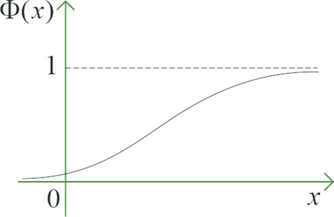
From Axiom 2, we have
Definition 5.
An UD
Definition 6.
Let
Definition 7.
An uncertain variable
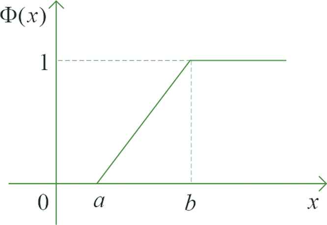
Linear uncertainty distribution.
The IUD of linear uncertain variable (LUV) Inverse linear uncertainty distribution.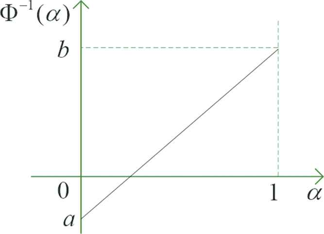
Theorem 1.
Let
2.2. Several Preference Relations
Let
2.2.1. Fuzzy preference relations
Definition 8.
[48] A FPR
Definition 9.
[49] The FPR
2.2.2. Interval fuzzy preference relations
Definition 10.
[50] Let
Definition 11.
[51] Let
Definition 12.
[1] Let
2.2.3. Incomplete fuzzy preference relations
Definition 13.
[10] Let
3. FPRs BASED ON UNCERTAINTY THEORY
3.1. Uncertain Preference Relations
Definition 14.
Let
Eq. (8) is the additive reciprocity of
For example, if
According to the additive reciprocity, Additive reciprocity of inverse LUD.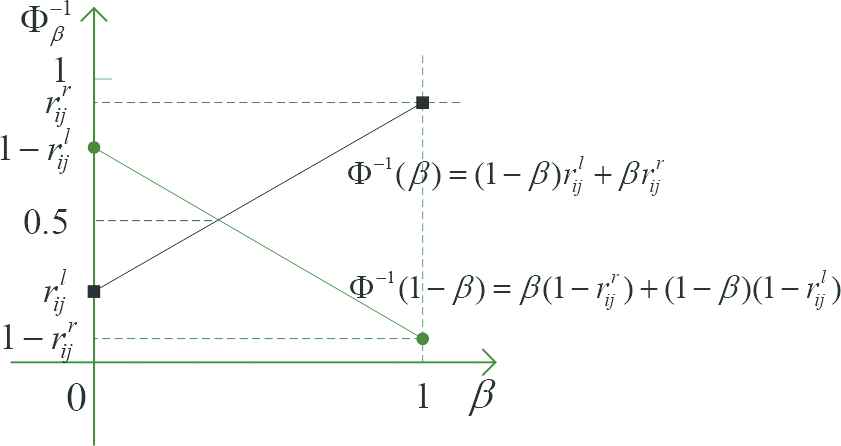
Definition 15.
Let
3.2. Uncertain Chance Constrained Programming Model
Let
In
For higher accuracy, the deviation between the ideal value
In the model,
Additionally,
Therefore, the equivalent model of
Let
Therefore, the equivalent model of
Theorem 2.
The linear equivalent model of UCCPM
3.3. Consistency Analysis of UPRs
3.3.1. Individual additive consistency analysis
Let
The smaller the value of
Definition 16.
[16] Let
The larger the
3.3.2. Adjustment of inconsistent UPRs
Definition 17.
Let
Theorem 3.
Let
Proof.
Thus,
Corollary 1.
Let
Proof.
Let
Since
In Corollary 1, after
3.3.3. Consensus analysis
To improve the level of consensus in GDM, all individual FPRs are typically aggregated to obtain a collective FPR. The latter is used to obtain the individual preference relation which deviates significantly from the consensus [4,52,53]. Combining the uncertainty theory and the aggregation operator, a consensus index which measures the deviation between an individual UPR and a collective UPR is introduced.
Let
Definition 18.
[16] Let
The smaller the
Since
IHWA Operator
Meng and Chen [16] propose an IHWA operator to calculate the elements of a collective FPR based on the importance of DMs (or criteria) and ordered positions. Extending the operator to interval UPRs, we propose the following definition of the collective UPR.
Definition 19.
[16] An IHWA operator with dimension n is a mapping IHWA: Let
Definition 20.
Let
Theorem 4.
Let
Proof.
From Eq. (13), we have
Weighted Averaging Consensus Index
Definition 21.
[16] Let
Theorem 5.
Let
Proof.
Based on Eq. (15), we have
Thus, the deviation after each adjustment is smaller than that of the previous one, namely, the consensus index of the UPR is better than that of the previous one.
An Algorithm for GDM
Step 1. Determine the preference relations and weight vectors.
Let
Step 2. Complete the incomplete UPRs.
Use UCCPM
Step 3. Calculate the individual consistency index.
Let
Step 4. Adjust inconsistent individual UPRs.
Let
Step 5. Calculate the individual consensus index.
Let
Step 6. Calculate the weighted averaging consensus index.
Use Eq. (18) to calculate the weighted averaging consensus index. If
Step 7. Adjust the individual UPRs.
Let
Step 8. Calculate the consistency index of the collective UPR.
Calculate the ultimate collective UPR
Step 9. Adjust inconsistent collective preference relation.
Let
3.4. Illustrative Example
Let
The incomplete UPRs
Step 1. Let the belief degree
Step 2. Let the individual ACI threshold value
Step 3. Let the consensus threshold value
e.g.,
Step 4. From Eq. (15),
Step 5. As
Let the ACI threshold value of the collective UPR be
To verify the feasibility and efficiency of the proposed method, comparative analysis is conducted using existing methods to estimate the missing values and calculate ACI.
Let
Meng et al. [54] propose the concepts of quasi intervals with its additive consistency presentation. It is independent of the permutation of object labels and considers the additive consistency of lower and upper endpoints of IPRs simultaneously. Further, Meng et al. [55] discover that the additive consistency of quasi intervals is included in Krejčí's [56] which is more flexible.
Using model (26) in [54] whose solutions of missing values has the highest additive consistency level with respect to known values and model (M-3) in [55] separately, the results are shown in Table 1. Although the proposed method is dependent on the labels of objects, the estimated values of proposed method are all included in the results of [54,55] when the belief degree
| Methods | Consistency | Missing Values |
ACI | ||||
|---|---|---|---|---|---|---|---|
| Method of Meng et al. [54] | Quasi intervals additive consistency | 0.6 | 0.3 | 0.63 | 0.1 | 0.43 | 0.893 |
| Method of Meng et al. [55] | Krejčí's additive consistency | 0.65 | 0.6 | 0.6 | 0.25 | 0.4 | 0.918 |
| The proposed method with |
UPRs additive consistency | 0.75 | 0.62 | 0.62 | 0.55 | 0.43 | 0.919 |
| The proposed method with |
UPRs additive consistency | 0.75 | 0.65 | 0.65 | 0.55 | 0.3 | 0.909 |
| The proposed method with |
UPRs additive consistency | 0.75 | 0.65 | 0.65 | 0.55 | 0.3 | 0.909 |
Determined missing values with different methods.
4. CONCLUSION
Based on the LUD and its consistency condition, the algorithm to fill in the incomplete values and the optimisation of group consistency of completed UPRs are investigated in this study.
The main contributions of this study are as follows:
An UCCPM is introduced to calculate the missing values in incomplete UPRs, which allows DMs to measure the confidence level of deviation between the supplementary values and the original incomplete information and guarantees the effectiveness of estimated values via a belief degree. It also proves that the operation of incomplete UPRs is an extension of that of traditional IPRs under a certain belief degree.
A novel distance measure and the ACI of incomplete UPRs are proposed to calculate the consistency and consensus degree of preference relations based on LUD. They are also used to improve the consistency and consensus index of UPRs iteratively.
The interval preference is treated collectively by obeying the LUD, which avoids the decision distortion and discretisation operation of intervals in the traditional interval operation.
Our future research will focus on two aspects. We discuss the situation of independent DMs in current work. If social relationships of individuals are considered, then GDM can be more scientific. Besides the interval preference information of DMs obeys a LUD, it may obey a NUD, zigzag uncertainty distribution, or lognormal uncertainty distribution, etc. Nonlinear distributions of other types of preference relations with their multiplicative consistency indices will be further investigated.
CONFLICT OF INTEREST
Authors have no conflict of interest to declare.
AUTHORS' CONTRIBUTIONS
The study is guided by Zaiwu Gong and written by all authors.
Funding statement
This work is supported in part by the National Natural Science Foundation of China under Grant 71971121, 71571104, 71871121 and 71401078, in part by the NUIST-UoR International Research Institute, in part by the Major Project Plan of Philosophy and Social Sciences Research in Jiangsu Universities under Grant 2018SJZDA038, in part by the 2019 Jiangsu Province Policy Guidance Program (Soft Science Research) under Grant BR2019064.
ACKNOWLEDGMENTS
Thank reviewers and editors for their valuable suggestions.
REFERENCES
Cite this article
TY  - JOUR
AU  - Xiujuan Ma
AU  - Zaiwu Gong
AU  - Weiwei Guo
PY  - 2020
DA  - 2020/01/30
TI  - Optimisation of Group Consistency for Incomplete Uncertain Preference Relation
JO  - International Journal of Computational Intelligence Systems
SP  - 130
EP  - 141
VL  - 13
IS  - 1
SN  - 1875-6883
UR  - https://doi.org/10.2991/ijcis.d.200121.002
DO  - 10.2991/ijcis.d.200121.002
ID  - Ma2020
ER  -