Interval-Valued Probabilistic Dual Hesitant Fuzzy Sets for Multi-Criteria Group Decision-Making

Peide Liu; Shufeng Cheng

doi:10.2991/ijcis.d.191119.001

<Previous Article In Issue

Download article (PDF)

Next Article In Issue>

Volume 12, Issue 2, 2019, Pages 1393 - 1411

Interval-Valued Probabilistic Dual Hesitant Fuzzy Sets for Multi-Criteria Group Decision-Making

Authors

Peide Liu^*, Shufeng Cheng

School of Management Science and Engineering, Shandong University of Finance and Economics, Jinan Shandong 250014, China

^*Corresponding author. Email: peide.liu@gmail.com

Corresponding Author

Peide Liu

Received 2 August 2019, Accepted 7 November 2019, Available Online 6 December 2019.

DOI: 10.2991/ijcis.d.191119.001 How to use a DOI?
Keywords: Interval-valued probabilistic dual hesitant fuzzy sets; Multi-criteria group decision-making; Ordered weighted averaging operator; Ordered distance and similarity measures; Risk evaluation
Abstract: As a powerful extension to hesitant fuzzy sets (HFSs), dual hesitant fuzzy sets (DHFSs) have been closely watched by many scholars. The DHFSs can reflect the disagreement and hesitancy of decision-makers (DMs) flexibly and conveniently. However, all the evaluation values under the same membership degree are endowed with similar importance. And DHFSs are not able to express DMs' preference degrees on different variables. To overcome this drawback, in this paper, we propose the concept of interval-valued probabilistic dual hesitant fuzzy sets (IVPDHFSs) by providing each element with an interval-valued probability value, which can describe DMs' preferences, hesitancy and disapproval simultaneously. Then we define the basic operation laws, score function and deviation function for interval-valued probabilistic dual hesitant fuzzy elements (IVPDHFEs). Besides, the ordered distance and similarity measures are proposed to calculate the deviation of any two IVPDHFSs and to derive the weight vector for DMs objectively, respectively. To aggregate decision-making information, we present interval-valued probabilistic dual hesitant fuzzy ordered weighted averaging (IVPDHFOWA) operator. Moreover, the water-filling theory is first introduced into IVPDHFSs environment and utilized to obtain unified criteria weights mathematically. Furthermore, a three-phased multi-criteria group decision-making (MCGDM) framework is constructed to address IVPDHFSs information. Finally, a case study concerning Arctic risk evaluation is provided to verify the effectiveness and superiority of the proposed three-phased framework.
Copyright: © 2019 The Authors. Published by Atlantis Press SARL.
Open Access: This is an open access article distributed under the CC BY-NC 4.0 license (http://creativecommons.org/licenses/by-nc/4.0/).

1. INTRODUCTION

The process of multi-criteria decision-making (MCDM) [1–5] is usually uncertain and complex in human activities. But how to deal with these vague issues is a challenging question. It is intractable to employ traditional techniques to cope with imprecise information. As a result, Zadeh [6] proposes the fuzzy sets (FSs) theory, which is generally recognized as a convenient model to describe imperfect and uncertain information [7]. FSs have only single membership function to describe the degree to which the given alternative satisfies the DMs. However, to express DMs' hesitancy on the performance of the given alternative, the corresponding models of FSs are limited. To alleviate this issue, Torra [8] introduces the concept of hesitant fuzzy sets (HFSs). Because HFSs allow several values to reflect the membership degree to which an element belongs to the given set, it is very suitable to use HFSs to express the hesitancy of DMs in the decision-making process.

Since HFSs have unique advantages, many scholars pay attention to the study of HFSs theory and obtain many achievements. On the theories of HFSs, Xu and Xia [9] investigate the aforementioned information measures and further define the ordered weighted distance and similarity measures for HFSs; Zhu et al. [10] apply proposed hesitant fuzzy geometric Bonferroni mean (HFGBM), hesitant fuzzy Choquet geometric Bonferroni mean (HFCGBM), weighted hesitant fuzzy geometric Bonferroni mean (WHFGBM) and weighted hesitant fuzzy Choquet geometric Bonferroni mean (WHFCGBM) to make MCDM; Zhang [11] develop a wide range of hesitant fuzzy power aggregation operators to aggregate input arguments that take the form of HFSs; Rodríguez et al. [12] make a position and perspective analysis of HFSs and a discussion about current proposals; Wei [13] proposes some prioritized aggregation operators to address MCDM problems in which the criteria are in different priority level; Xu and Zhang [14] develop a new approach based on TOPSIS and maximizing deviation method to handle hesitant fuzzy information. Moreover, there are some successful extensions of HFSs, such as hesitant fuzzy linguistic term sets [15,16], interval-valued HFSs [17,18], interval-valued hesitant fuzzy linguistic sets [19], interval-valued intuitionistic HFSs [20,21], DHFSs [22], generalized HFSs [23], triangular HFSs [24], probabilistic HFSs (PHFSs) [25] and interval-valued PHFSs (IVPHFSs) [26,27].

Among all the extensions of HFSs, DHFSs have gained wide popularity since it can depict the membership hesitancy degree and non-membership hesitancy degree in the domain simultaneously. Ye [28] proposes a correlation coefficient of DHFSs and apply it to solve MCDM problems. Su et al. [29] introduce the distance and similarity measures for DHFSs. Based on Archimedean t-conorm and t-norm, Wang et al. [30] present some dual hesitant fuzzy power aggregation operators for multiple criteria group decision-making (MCGDM). Singh [31] presents a new similarity measure and further proposes two algorithms to find the optional solution under DHFSs environments. Wang et al. [32] introduce generalized dual hesitant fuzzy Choquet ordered aggregation (GDHFCOA) operator for MCDM. Ren et al. [33] propose a comparison method to distinguish DHFSs efficiently and extend the VIKOR method into DHFSs environment for MCGDM. Yu and Li [34] apply the generalized dual hesitant fuzzy weighted averaging (GDHFWA) operator, the generalized dual hesitant fuzzy ordered weighted averaging (GDHFOWA) operator and the generalized dual hesitant fuzzy hybrid averaging (GDHFHA) operator to aggregate dual hesitant fuzzy information. Yu et al. [35] propose dual hesitant fuzzy Heronian mean operator and dual hesitant fuzzy geometric Heronian mean operator and utilize them to make group decision-making (GDM) for supplier selection. Zhao et al. [36] introduce dual hesitant fuzzy preference relation (DHFPR), which provides a powerful solution to describe the hesitant cognitions of DMs over some feasible alternatives. Ren and Wei [37] employ the proposed correctional score function and the dice similarity measure for DHFSs to address MCDM problems in which the attributes are in different priority levels.

Though these operators and methods can handle dual hesitant fuzzy information effectively, still the issue of DMs' preference on evaluation values has not been addressed. In the membership degree part or the non-membership degree part of DHFSs, all elements have the same importance or weight. Apparently, it is not in conformity in real life. DMs may prefer one element to another one due to the epistemic uncertainty. Up to now, probabilistic approaches are prevalent to model the aleatory uncertainty in terms of the statistical uncertainty but are unable to solve complex and fuzzy MCGDM problems. Thus, it is a hot academic issue that how to combine the randomness in mathematics and vagueness in complex MCDM problems efficiently, which motivates many scholars to make a large number of investigations.

On the whole, the work to incorporate probability theory into fuzzy sets theory can be roughly summarized into the following process: (i) introducing the probability theory and make it available in fuzzy sets theory; (ii) integrating the probability theory into fuzzy operation, measure and aggregation process and (iii) combined methods producing the probabilistic fuzzy values. Followed by this idea, the immediate probability was introduced into the fuzzy decision-making process [38,39]. The immediate probability information can reflect the attitudinal characteristics of DMs precisely and be properly considered as the weight information of the corresponding element in the aggregation process. To transform this incorporated theory into practical applications where the evaluation information is denoted by DHFSs, Hao et al. [40] propose the concept of probabilistic dual hesitant fuzzy sets (PDHFSs) and define the operational laws and some aggregation operators for PDHFSs. In the probabilistic dual hesitant fuzzy element (PDHFE), each evaluation value is endowed with an occurring probability to express the confidence and preference of DMs. Meanwhile, Zeng et al. [41] present the concept of weighted dual hesitant fuzzy sets (WDHFSs) and weighted dual hesitant fuzzy element (WDHFE) and provide a GDM method under DHFSs environment. For instance, an expert is invited to assess the performance of a central processing unit (CPU) manufacturing company over the technical ability attribute, he/she provide a dual hesitant fuzzy element (DHFE) 〈0.4,0.6,0.8,0.2,0.3〉 due to the hesitancy character. Nevertheless, he/she has more confidence in the value 0.6 in the satisfaction degree function and the value 0.2 in the dissatisfaction degree function, which is beyond the scope of DHFSs. But PDHFSs and WDHFSs can describe this preference information perfectly. Supposing the weights for 0.4,0.6,0.8 in the membership degree are 0.2,0.6,0.2 respectively and the weights for 0.2,0.3 in the non-membership degree are 0.7,0.3 respectively, his/her comment on this statement can be denoted as 〈0.40.2,0.60.6,0.80.2,0.20.7,0.30.3〉.

However, we may ignore the fact that DMs are unable to give precise probability preference information for their comments. In some real scenarios, DMs may estimate the preference degree of a certain membership value using linguistic form or interval format. It is unreasonable and irrational to utilize PDHFSs and WDHFSs to express linguistic or interval preference information. As a result, we propose the concept of interval-valued probabilistic dual hesitant fuzzy sets (IVPDHFSs), in which the occurring probability of each element in satisfaction and dissatisfaction degrees is extended to a range covering lower and upper limit values. By contrast, IVPDHFSs are quite suitable to reflect the uncertain preference degree in the decision-making process. Some motivations for this research are summarized as follows:

PDHFSs cannot express DMs' hesitant probabilistic preference. Motivated by this weakness, we are devoted to presenting a new concept called IVPDHFSs, which allocates each element with an interval-valued probability value.
Motivated by the rationality and consistency of aggregation operator, efforts are made to utilize ordered weight averaging operator to fuse IVPDHFSs information.
Motivated by the effectiveness and practicability of score function and deviation function of HFSs, contributions are made to extend score and deviation functions in IVPDHFSs environment.
Motivated by the risk preference character of DMs, we propose ordered distance and similarity measures to calculate the difference of any two IVPDHFSs.
A large number of models for deriving the criteria weights rarely take the criteria dimensions into account. Motivated by the power of water-filling theory, the achievement is made to remove the influence of criteria dimensions and magnitude the criteria into a consistent scale.
Motivated by the efficiency and flexibility of interval-valued probabilistic preference, we regard IVPDHFSs as a novel basic theory and further put forward a three-phased MCGDM framework under IVPDHFSs environment.

Some main contributions of this paper are presented below:

We define a new concept of IVPDHFSs so as to describe the hesitant probabilistic preference of DMs.
We propose the operational laws for IVPDHFEs and further present the IVPDHFOWA operator to make information fusion.
The score function and deviation function is defined to make a simple comparison of any two IVPDHFEs.
We present the ordered distance measure to compute the difference of any IVPDHFEs and introduce the ordered similarity measure to derive the weight vector of DMs.
The water-filling theory is first introduced into IVPDHFSs environment, and based on this theory, we construct a mathematical model to derive the criteria weights, which eliminates the impact of criteria dimensions.
A three-phased MCGDM framework is conceived to handle IVPDHFSs information.

The organization of this paper is constructed as follows. In Section 2, we review some definitions of HFSs, DHFSs and PDHFSs. In Section 3, we give a series of concepts of IVPDHFSs and propose the operational laws and comparison method for IVPDHFEs. Besides, the ordered distance and similarity measures and IVPDHFOWA operator are also presented. In Section 4, we propose a three-phased MCGDM framework within IVPDHFSs. In Section 5, we make a case study to verify the validity of the proposed three-phased framework. Finally, a conclusion is provided in Section 6.

2. PRELIMINARIES

In this section, we review some conceptions related to HFSs, DHFSs and PDHFSs.

2.1. Hesitant Fuzzy Sets

Definition 1.

[8] An HFS H on the reference set X is defined in terms of a membership function hx that returns a subset of 0,1 when applied to X.

Xia and Xu [42] provide the mathematical symbol of HFS as follows:

(1)H=〈x,hx〉|x∈X,

where hx is a set of several possible values in interval 0,1. For convenience, hx is called a hesitant fuzzy element (HFE).

2.2. Dual Hesitant Fuzzy Sets

Definition 2.

[22] A DHFS D on the reference set X is defined in terms of the membership hesitancy function hx and non-membership hesitancy function gx that both return a set of 0,1 when applied to X. Mathematically, it can be expressed by the following symbol:

(2)D=〈x,hx,gx〉|x∈X,

where hx and gx satisfy the following conditions: ∀x∈X, γ≥0, η≤1, 0≤γ++η+≤1, γ∈hx, η∈gx, γ+=∪γ∈hxmaxγ and η+=∪η∈gxmaxη. For simplicity, the pair 〈hx,gx〉 is called a dual hesitant fuzzy element (DHFE).

Zhu et al. [22] also give basic operations for DHFSs.

Definition 3.

[22] Let d=h,g, d1=h1,g1 and d2=h2,g2 be any three DHFEs, then the operational laws are as follows:

(3)⊕−union:d1⊕d2=h1⊕h2,g1⊗g2 =∪γ1∈h1,γ2∈h2η1∈g1,η2∈g2γ1+γ2−γ1γ2,η1η2;

(4)⊗−intersection:d1⊗d2=h1⊗h2,g1⊕g2=∪γ1∈h1,γ2∈h2η1∈g1,η2∈g2γ1γ2,η1+η2−η1η2;

(5)λd=∪γ∈h,η∈g1−1−γλ,ηλ,λ≥0;

(6)dλ=∪γ∈h,η∈gγλ,1−1−ηλ,λ≥0.

2.3. Probabilistic Dual Hesitant Fuzzy Sets

Definition 4.

[40] A PDHFS P on the reference set X is defined as the following symbol:

(7)P=〈x,hx|px,gx|qx〉|x∈X,

where hx and gx represent the membership hesitancy function and non-membership hesitancy function, respectively. px and qx denote the corresponding single probability value for the elements in these two possible degrees. Besides, the two parts hx|px and gx|qx satisfy the following conditions: ∀x∈X, γ≥0, η≤1, 0≤γ++η+≤1, γ∈hx, η∈gx, γ+=∪γ∈hxmaxγ, η+=∪η∈gxmaxη, px∈0,1, qx∈0,1, ∑pi∈pxpi=1 and ∑qj∈qxqj=1. For the sake of convenience, the pair 〈hx|px,gx|qx〉 is called as a PDHFE.

Hao et al. [40] also give the basic operational laws for PDHFSs as follows:

Definition 5.

[40] Let P=h|p,g|q, P1=h1|p1,g1|q1, P2=h2|p2,g2|q2 be three PDHFEs, then

(8)P1⊕P2=h1⊕h2,g1⊗g2 =∪γ1∈h1,γ2∈h2,pγ1∈p1,pγ2∈p2η1∈g1,η2∈g2,qη1∈q1,qη2∈q2 γ1+γ2−γ1γ2|pγ1pγ2,η1η2|qη1qη2;

(9)P1⊗P2=h1⊗h2,g1⊕g2 =∪γ1∈h1,γ2∈h2,pγ1∈p1,pγ2∈p2η1∈g1,η2∈g2,qη1∈q1,qη2∈q2 γ1γ2|pγ1pγ2,η1+η2−η1η2|qη1qη2;

(10)λP=∪γ∈h,pr∈pη∈g,qη∈q1−1−γλ|pr,ηλ|qη,λ≥0;

(11)Pλ=∪γ∈h,pr∈pη∈g,qη∈qγλ|pr,1−1−ηλ|qη,λ≥0.

3. INTERVAL-VALUED PROBABILISTIC DUAL HESITANT FUZZY SETS

In this section, to describe the probabilistic hesitant information flexibly and reasonably, we propose the concept of IVPDHFSs and investigate basic operational laws and its comparison method. Besides, we define the ordered distance and similarity measures of generalized IVPDHFSs. To fuse information, the interval-valued probabilistic dual hesitant fuzzy ordered weighted averaging (IVPDHFOWA) operator is presented.

3.1. The Concept of IVPDHFSs

As has been discussed above, it is difficult for the DMs to give precise probabilistic preference degrees on their evaluation values. Sometimes, they prefer to use interval-valued probability to express their opinions instead of single-valued probability. Thus, we present the concept of IVPDHFSs as follows:

Definition 6.

Let X be the reference set, an IVPDHFS on X is defined by the following expression:

(12)DIVP=〈x,hx|plx,pux,g(x)|qlx,qux〉|x∈X.

The components hx|plx,pux and gx|qlx,qux are the two distinct membership functions, in which hx and gx are the satisfaction function and dissatisfaction function of x to the set of X, respectively, plx,pux and qlx,qux are the interval probabilistic preference values corresponding to membership functions hx and gx, respectively, satisfying γ≥0, η≤1, 0≤γ++η+≤1, γ∈hx, η∈gx, γ+=∪γ∈hxmaxγ, η+=∪η∈gxmaxη, 0≤pγl≤1, 0≤pγu≤1, pγl≤pγu, 0≤qηl≤1, 0≤qηu≤1, qηl≤qηu, pγl,pγu∈plx,pux, qηl,qηu∈qlx,qux, ∑pγu∈puxpγu≤1 and ∑qηu∈quxqηu≤1 for any x∈X.

For the sake of simplicity, the pair 〈x,hx|plx,pux,gx|qlx,qux〉 is called as interval-valued probabilistic dual hesitant fuzzy element (IVPDHFE), and simply denoted by dIVP=h|phl,phu,g|qgl,qgu.

In real problems, some evaluation values may be lost due to complex decision-making environment and unexpected ignorance behaviors. Thus, we provide the definition of generalized IVPDHFSs and discuss some special forms of IVPDHFSs.

Definition 7.

Let DIVP=〈x,hx|plx,pux,gx|qlx,qux〉|x∈X be an IVPDHFS, if #hx≥2, #gx≥2, plx<pux and qlx<qux, where #hx and #gx denote the total numbers of the elements in membership function hx and non-membership function gx, respectively, then we call DIVP generalized IVPDHFS. For short, generalized IVPDHFS is also denoted as DIVP.

Remark 1.

Let DIVP=〈x,hx|plx,pux,gx|qlx,qux〉|x∈X be an IVPDHFS, if #hx≥2, #gx≥2, plx=pux and qlx=qux, where #hx and #gx denote the total numbers of the elements in membership function hx and non-membership function gx, respectively, then IVPDHFS is reduced to PDHFS; if #hx≥2, gx=∅ and plx<pux, where #hx denotes the total number of the elements in membership function hx, then IVPDHFS is reduced to IVPHFS; if #hx≥2, gx=∅ and plx=pux, where #hx denotes the total number of the elements in membership function hx, then IVPDHFS reduces to PHFS.

Very often in the decision-making process, the elements in given IVPDHFEs are disordered, which may lead to difficulties in operation. Thus, we propose the concept of ordered IVPDHFE as follows:

Definition 8.

Let dIVP=h|phl,phu,g|qgl,qgu be a generalized IVPDHFE, if the elements ∪γ∈hγ in membership function h are sorted based on the values of γpγl2+pγu2 in descending order and the elements ∪η∈gη in membership function g are sorted based on the values of ηqηl2+qηu2 in descending order, then this IVPDHFE is called an ordered IVPDHFE.

Remark 2.

Specially, if the values of γpγl2+pγu2 are equal, then the elements ∪γ∈hγ in membership function h are sorted based on the values of γ in descending order. And if the values of ηqηl2+qηu2 are equal, then the elements ∪η∈gη in membership function g are sorted based on the values of η in descending order.

Example 1.

Given an IVPDHFE dIVP=〈0.8|0.2,0.3,0.6|0.5,0.7,0.6|0.3,0.4,0.4|0.3,0.6〉, if we calculate and line up the values of γpγl2+pγu2 and ηqηl2+qηu2, respectively, then a new IVPDHFE is acquired. Since 0.8×0.22+0.32=0.104, 0.6×0.52+0.72=0.444, 0.6×0.32+0.42=0.15 and 0.4×0.32+0.62=0.18, the new IVPDHFE d˙IVP=〈0.6|0.5,0.7,0.8|0.2,0.3,0.4|0.3,0.6,0.6|0.3,0.4〉 is an ordered IVPDHFE.

For an IVPDHFE dIVP=h|phl,phu,g|qgl,qgu, if ∑pγu∈phupγu=1 and ∑qηu∈qguqηu=1, then the probability distribution of all elements is complete; if ∑pγu∈phupγu<1 or ∑qηu∈qguqηu<1, then the probability distribution of all elements is incomplete, namely, some probabilistic information is lost and ignored. To overcome this cognitive limitation, we give the concept of normalized IVPDHFSs.

Definition 9.

Let DIVP=〈x,hx|plx,pux,gx|[ql(x),qu(x)]⟩|x∈X} be an IVPDHFS, then its normalized form is denoted by

(13)D¯IVP=〈x,hx|p¯lx,p¯ux,gx|q¯lx,q¯ux〉|x∈X,

where the elements pγl,pγu∈plx,pux and qηl,qηu∈qlx,qux are normalized as

(14)p¯γl=pγl∑pγl∈plx,pγu∈puxpγl2+pγu22,

(15)p¯γu=pγu∑pγl∈plx,pγu∈puxpγl2+pγu22,

(16)q¯ηl=qηl∑qηl∈qlx,qηu∈quxqηl2+qηu22,

(17)q¯ηu=qηu∑qηl∈qlx,qηu∈quxqηl2+qηu22.

3.2. The Basic Operations for IVPDHFSs

Definition 10.

(18)dIVP1⊕dIVP2=∪γ1∈h1,γ2∈h2,η1∈g1,η2∈g2pγ1l∈ph1l,pγ1u∈ph1u,pγ2l∈ph2l,pγ2u∈ph2uqη1l∈qg1l,qη1u∈qg1u,qη2l∈qg2l,qη2u∈qg2u γ1+γ2−γ1γ2|pγ1lpγ2l,pγ1upγ2u,η1η2|qη1lqη2l,qη1uqη2u;

(19)dIVP1⊗dIVP2=∪γ1∈h1,γ2∈h2,η1∈g1,η2∈g2pγ1l∈ph1l,pγ1u∈ph1u,pγ2l∈ph2l,pγ2u∈ph2uqη1l∈qg1l,qη1u∈qg1u,qη2l∈qg2l,qη2u∈qg2u γ1γ2|pγ1lpγ2l,pγ1upγ2u,η1+η2−η1η2|qη1lqη2l,qη1uqη2u;

(20)λdIVP=∪γ∈h,η∈gpγl∈phl,pγu∈phuqηl∈qgl,qηu∈qgu1−1−γλ|pγl,pγu,ηλ|qηl,qηu,λ≥0;

(21)dIVPλ=∪γ∈h,η∈gpγl∈phl,pγu∈phuqηl∈qgl,qηu∈qguγλ|pγl,pγu,1−1−ηλ|qηl,qηu,λ≥0;

(22)dIVPc=∪γ∈h,η∈gpγl∈phl,pγu∈phuqηl∈qgl,qηu∈qguη|qηl,qηu,γ|pγl,pγu.

Remark 3.

In IVPDHFSs, the probability distribution of all elements is denoted by interval values with lower limits and upper limits. For each evaluation value, if the lower limit is equal to the upper limit, namely, interval-valued probability reduces to single probability, then Eqs. (18–21) reduce to Eqs. (8–11); if all the elements in membership set and non-membership set have equal importance and weight, namely, phl=phu=1#h, qgl=qgu=1#g, where #h and #g represent the total numbers of all elements in membership function and non-membership function, respectively, then balanced probability information cannot reflect preference character of DMs, and Eqs. (18–21) reduce to Eqs. (3–6).

Property 1.

The complement set of generalized IVPDHFS is involutive.

Proof.

According to the Eq. (22), we can conclude that

Property 2.

Commutative

(23)dIVP1⊕dIVP2=dIVP2⊕dIVP1;

(24)dIVP1⊗dIVP2=dIVP2⊗dIVP1;

Property 3.

Associative

(25)dIVP1⊕dIVP2⊕dIVP3=dIVP1⊕dIVP2⊕dIVP3;

(26)dIVP1⊗dIVP2⊗dIVP3=dIVP1⊗dIVP2⊗dIVP3;

Proof.

The proofs for Properties 2 and 3 are straightforward and simple. Here, we concrete on these Properties alone.

Property 4.

Distributive

(27)λdIVP1+dIVP2=λdIVP1+λdIVP2,λ≥0;

(28)λ1+λ2dIVP=λ1dIVP+λ2dIVP,λ1,λ2≥0;

Proof.

For the left part of Eq. (27), we have

λdIVP1+dIVP2=λ∪γ1∈h1,γ2∈h2η1∈g1,η2∈g2pγ1l∈ph1l,pγ1u∈ph1upγ2l∈ph2l,pγ2u∈ph2uqη1l∈qg1l,qη1u∈qg1uqη2l∈qg2l,qη2u∈qg2uγ1+γ2−γ1γ2|pγ1lpγ2l,pγ1upγ2u,η1η2|qη1lqη2l,qη1uqη2u =λ∪γ1∈h1,γ2∈h2η1∈g1,η2∈g2pγ1l∈ph1l,pγ1u∈ph1upγ2l∈ph2l,pγ2u∈ph2uqη1l∈qg1l,qη1u∈qg1uqη2l∈qg2l,qη2u∈qg2u1−1−γ11−γ2|pγ1lpγ2l,pγ1upγ2u,η1η2|qη1lqη2l,qη1uqη2u =∪γ1∈h1,γ2∈h2η1∈g1,η2∈g2pγ1l∈ph1l,pγ1u∈ph1upγ2l∈ph2l,pγ2u∈ph2uqη1l∈qg1l,qη1u∈qg1uqη2l∈qg2l,qη2u∈qg2u1−1−γ1λ1−γ2λ|pγ1lpγ2l,pγ1upγ2u,η1 λη2 λ|qη1lqη2l,qη1uqη2u

For the right part of Eq. (27), we have

λdIVP1+λdIVP2=∪γ1∈h1,η1∈g1pγ1l∈ph1l,pγ1u∈ph1uqη1l∈qg1l,qη1u∈qg1u1−1−γ1λ|pγ1l,pγ1u,η1 λ|qη1l,qη1u +∪γ2∈h2,η2∈g2pγ2l∈ph2l,pγ2u∈ph2uqη2l∈qg2l,qη2u∈qg2u1−1−γ2λ|pγ2l,pγ2u,η2 λ|qη2l,qη2u =∪γ1∈h1,γ2∈h2η1∈g1,η2∈g2pγ1l∈ph1l,pγ1u∈ph1upγ2l∈ph2l,pγ2u∈ph2uqη1l∈qg1l,qη1u∈qg1uqη2l∈qg2l,qη2u∈qg2u1−1−γ1λ+1−1−γ2λ−1−(1−γ1)λ1−(1−γ2)λ|pγ1lpγ2l,pγ1upγ2u,η1 λη2 λ|qη1lqη2l,qη1uqη2u =∪γ1∈h1,γ2∈h2η1∈g1,η2∈g2pγ1l∈ph1l,pγ1u∈ph1upγ2l∈ph2l,pγ2u∈ph2uqη1l∈qg1l,qη1u∈qg1uqη2l∈qg2l,qη2u∈qg2u1−1−γ1λ1−γ2λ|pγ1lpγ2l,pγ1upγ2u,η1 λη2 λ|qη1lqη2l,qη1uqη2u.

Thus, Eq. (27) is kept.

Similarly, Eq. (28) can be proved.

Theorem 1.

All the results acquired from Eqs. (18–28) are also IVPDHFSs.

Proof.

The proof is easy and straightforward.

Theorem 2.

(29)dIVP1λ×dIVP2λ=dIVP1×dIVP2λ,λ≥0;

(30)dIVPλ1×dIVPλ2=dIVPλ1+λ2,λ1,λ2≥0.

Proof.

For the left part of Eq. (29), we have

dIVP1λ×dIVP2λ=∪γ1∈h1,η1∈g1pγ1l∈ph1l,pγ1u∈ph1uqη1l∈qg1l,qη1u∈qg1uγ1λ|pγ1l,pγ1u,1−1−η1λ|qη1l,qη1u ×∪γ2∈h2,η2∈g2pγ2l∈ph2l,pγ2u∈ph2uqη2l∈qg2l,qη2u∈qg2uγ2λ|pγ2l,pγ2u,1−1−η2λ|qη2l,qη2u =∪γ1∈h1,γ2∈h2,η1∈g1,η2∈g2pγ1l∈ph1l,pγ1u∈ph1u,pγ2l∈ph2l,pγ2u∈ph2uqη1l∈qg1l,qη1u∈qg1u,qη2l∈qg2l,qη2u∈qg2uγ1λγ2λ|pγ1lpγ2l,pγ1upγ2u,1−1−η1λ+1−1−η2λ−1−1−η1λ1−1−η2λ|qη1lqη2l,qη1uqη2u =∪γ1∈h1,γ2∈h2,η1∈g1,η2∈g2pγ1l∈ph1l,pγ1u∈ph1u,pγ2l∈ph2l,pγ2u∈ph2uqη1l∈qg1l,qη1u∈qg1u,qη2l∈qg2l,qη2u∈qg2uγ1λγ2λ|pγ1lpγ2l,pγ1upγ2u,1−1−η1λ1−η2λ|qη1lqη2l,qη1uqη2u

For the right part of Eq. (29), we have

dIVP1×dIVP2λ=∪γ1∈h1,γ2∈h2,η1∈g1,η2∈g2pγ1l∈ph1l,pγ1u∈ph1u,pγ2l∈ph2l,pγ2u∈ph2uqη1l∈qg1l,qη1u∈qg1u,qη2l∈qg2l,qη2u∈qg2uγ1γ2|pγ1lpγ2l,pγ1upγ2u,η1+η2−η1η2|qη1lqη2l,qη1uqη2uλ =∪γ1∈h1,γ2∈h2,η1∈g1,η2∈g2pγ1l∈ph1l,pγ1u∈ph1u,pγ2l∈ph2l,pγ2u∈ph2uqη1l∈qg1l,qη1u∈qg1u,qη2l∈qg2l,qη2u∈qg2uγ1λγ2λ|pγ1lpγ2l,pγ1upγ2u,1−1−1−1−η11−η2λ|qη1lqη2l,qη1uqη2u =∪γ1∈h1,γ2∈h2,η1∈g1,η2∈g2pγ1l∈ph1l,pγ1u∈ph1u,pγ2l∈ph2l,pγ2u∈ph2uqη1l∈qg1l,qη1u∈qg1u,qη2l∈qg2l,qη2u∈qg2uγ1λγ2λ|pγ1lpγ2l,pγ1upγ2u,1−1−η1λ1−η2λ|qη1lqη2l,qη1uqη2u

Thus, Eq. (29) is kept.

Similarly, Eq. (30) can be proved.

Theorem 3.

(31)dIVP1c⊕dIVP2c=dIVP1⊗dIVP2c;

(32)dIVP1c⊗dIVP2c=dIVP1⊕dIVP2c;

(33)dIVPcλ=λdIVPc,λ≥0;

(34)λdIVPc=dIVPλc,λ≥0.

Proof.

For the left part of Eq. (31), we have

dIVP1c⊕dIVP2c=∪γ1∈h1,η1∈g1pγ1l∈ph1l,pγ1u∈ph1uqη1l∈qg1l,qη1u∈qg1uη1|qη1l,qη1u,γ1|pγ1l,pγ1u⊕∪γ2∈h2,η2∈g2pγ2l∈ph2l,pγ2u∈ph2uqη2l∈qg2l,qη2u∈qg2uη2|qη2l,qη2u,γ2|pγ2l,pγ2u =∪γ1∈h1,γ2∈h2η1∈g1,η2∈g2pγ1l∈ph1l,pγ1u∈ph1upγ2l∈ph2l,pγ2u∈ph2uqη1l∈qg1l,qη1u∈qg1uqη2l∈qg2l,qη2u∈qg2uη1+η2−η1η2|qη1lqη2l,qη1uqη2u,γ1γ2|pγ1lpγ2l,pγ1upγ2u,

and for the right part of Eq. (31), we have

dIVP1⊗dIVP2c=∪γ1∈h1,γ2∈h2,η1∈g1,η2∈g2pγ1l∈ph1l,pγ1u∈ph1u,pγ2l∈ph2l,pγ2u∈ph2uqη1l∈qg1l,qη1u∈qg1u,qη2l∈qg2l,qη2u∈qg2uγ1γ2|pγ1lpγ2l,pγ1upγ2u,η1+η2−η1η2|qη1lqη2l,qη1uqη2uc =∪γ1∈h1,γ2∈h2,η1∈g1,η2∈g2pγ1l∈ph1l,pγ1u∈ph1u,pγ2l∈ph2l,pγ2u∈ph2uqη1l∈qg1l,qη1u∈qg1u,qη2l∈qg2l,qη2u∈qg2uη1+η2−η1η2|qη1lqη2l,qη1uqη2u,γ1γ2|pγ1lpγ2l,pγ1upγ2u.

Thus, Eq. (31) is hold.

Similarly, Eqs. (32–34) can be proved.

3.3. The Comparison Method for IVPDHFEs

For an IVPDHFS, the elements in satisfaction function and dissatisfaction function are almost in the partial order. However, it is useful and necessary to rank a set of IVPFDHFEs in decision-making problems. Hence, we propose the score function and deviation function for IVPDHFEs, providing reliable access to the comparison of IVPDHFEs.

Definition 11.

Let dIVP=h|phl,phu,g|qgl,qgu be the generalized IVPDHFE, then the score function for IVPDHFE is expressed by the following mathematical symbol:

(35)sdIVP=∑γ∈h#hγpγl+γpγu−∑η∈g#gηqηl+ηqηu.

For any two generalized IVPDHFEs dIVP1 and dIVP2, if sdIVP1>sdIVP2, then the IVPDHFE dIVP1 is superior to the IVPDHFE dIVP2, mathematically denoted as dIVP1≻dIVP2; if sdIVP1<sdIVP2, then the IVPDHFE dIVP1 is inferior to the IVPDHFE dIVP2, mathematically denoted as dIVP1≺dIVP2; if sdIVP1=sdIVP2, then it is inappropriate to draw the conclusion that these two IVPDHFEs are equal and identical. In this situation, another indicator is needed, thus, we define the deviation function for IVPDHEs to make a further comparison.

Definition 12.

Let dIVP=h|phl,phu,g|qgl,qgu be the generalized IVPDHFE, then the deviation function for IVPDHFE is denoted by the following expression:

(36)σdIVP=∑γ∈h#hγ−sdIVP2pγl+pγu +∑η∈g#gη−sdIVP2qηl+qηu12.

As expressed in Eq. (36), the deviation function σdIVP reflects the overall fluctuation degree of an IVPDHFE from the average level. The smaller value of σdIVP implies higher coherence while the bigger value of σdIVP indicates lower coherence.

Considering the score function and deviation function for IVPDHFEs, we further present the comparison method for IVPDHFEs.

Definition 13.

Let dIVP1=h1|ph1l,ph1u,g1|qg1l,qg1u, dIVP2=h2|ph2l,ph2u,g2|qg2l,qg2u be any two generalized IVPDHFEs, then

If sdIVP1>sdIVP2, then the IVPDHFE dIVP1 is superior to the IVPDHFE dIVP2, mathematically denoted as dIVP1≻dIVP2.
If sdIVP1<sdIVP2, then the IVPDHFE dIVP1 is inferior to the IVPDHFE dIVP2, mathematically denoted as dIVP1≺dIVP2.
If sdIVP1=sdIVP2, then
1. if σdIVP1<σdIVP2, then the IVPDHFE dIVP1 is superior to the IVPDHFE dIVP2, mathematically denoted as dIVP1≻dIVP2.
2. if σdIVP1>σdIVP2, then the IVPDHFE dIVP1 is inferior to the IVPDHFE dIVP2, mathematically denoted as dIVP1≺dIVP2.
3. if σdIVP1=σdIVP2, then the IVPDHFE dIVP1 is equivalent to the IVPDHFE dIVP2, mathematically denoted as dIVP1∼dIVP2.

3.4. The Ordered Distance and Similarity Measures for Generalized IVPDHFSs

The distance and similarity measures are classical tools to address decision-making problems in which the evaluation on alternative projects is denoted by FSs, HFSs, DHFSs and PHFSs. These measures can also reflect the closeness degree of any two items easily in practical applications. Hence, it is essential to study the distance and similarity measures under IVPDHFSs environment. To this end, we introduce the axioms for distance and similarity measures for IVPDHFSs.

Definition 14.

Let M and N be two generalized IVPDHFSs on the reference set X, then the distance measure between M and N is expressed as dM,N, satisfying the following properties:

0≤dM,N≤1;
dM,N=0 if and only if M=N;
dM,N=dN,M=dMc,Nc=dNc,Mc.

Definition 15.

Let M and N be two generalized IVPDHFSs on the reference set X, then the similarity measure between M and N is expressed as sM,N, satisfying the following properties:

0≤sM,N≤1;
sM,N=1 if and only if M=N;
sM,N=sN,M=sMc,Nc=sNc,Mc.

Since there are complement relationships between the distance measure and the similarity measure, we mainly concrete on the distance measure of IVPDHFSs, and the similarity measure for IVPDHFSs can be obtained easily.

In most circumstance, for any x∈X, #hMx≠#hNx or #gMx≠#gNx, namely, the membership sets or non-membership sets in two IVPDHFSs have unequal length. Inspired by the idea of Xu and Xia [9] and Liu et al. [43], we propose the ordered distance measure for IVPDHFSs,

where σi, σj, σs and σt are the i-th, j-th, s-th and t-th largest values in corresponding sets, respectively.

Based on Eq. (37), we can obtain the distance measure for IVPDHFEs easily:

Remark 4.

Before measuring the distance between any two IVPDHFEs by utilizing Eq. (38), we need to make the following two-step preparation.

Firstly, we need to line up all the elements in IVPDHFEs in descending order by referring to the Definition 8.

Secondly, for the membership set, two IVPDHFEs may have unequal length. Hence, we need to extend the shorter membership set until both of them have equal length. There are many methods to extend the shorter one, such as adding some elements in it. In most cases, we almost add some same values at the end or beginning of the shorter one, which depends on the DMs' attitude towards possible risks. Optimistic DMs are willing to add the element γ|pγl,pγu with maximum value of γpγl2+pγu2 at the beginning of the shorter membership set until its length is equal to that of the longer membership set, while pessimistic DMs usually add the element γ|pγl,pγu with minimum value of γpγl2+pγu2 at the end of the shorter membership set until its length is equal to that of the longer membership set. It is also the same for the non-membership set.

According to the ordered distance measure for IVPDHFSs, the ordered similarity measure is denoted by the following expression:

3.5. Interval-Valued Probabilistic Dual Hesitant Fuzzy Ordered Weighted Averaging Operator

In fuzzy MCGDM problems, it is essential to fuse DMs' assessments into comprehensive information. Based on Definitions 8 and 10, we propose a basic aggregation operator under IVPDHFSs environment.

Definition 16.

Let dIVPi=hi|phil,phiu,gi|qgil,qgiui=1,2,⋯,n be a collection of IVPDHFEs, dIVPσi be the i-th largest element of them, and ω=ω1,ω2,⋯,ωnT be the associated weight vector such that 0≤ωi≤1 and ∑i=1nωi=1, then the IVPDHFOWA operator is a mapping IVPDHFOWA : Dn→D, where

(40)IVPDHFOWAdIVP1,dIVP2,⋯,dIVPn=⊕i=1nωidIVPσi=∪γ1∈hσ1,γ2∈hσ2,⋯,γn∈hσnη1∈gσ1,η2∈gσ2,⋯,ηn∈gσnpγ1l∈phσ1l,pγ1u∈phσ1u,pγ2l∈phσ2l,pγ2u∈phσ2u,⋯,pγnl∈phσnl,pγnu∈phσnuqη1l∈qgσ1l,qη1u∈qgσ1u,qη2l∈qgσ2l,qη2u∈qgσ2u,⋯,qηnl∈qgσnl,qηnu∈qgσnu 1−∏i=1n1−γiωi|∏i=1npγil,∏i=1npγiu,∏i=1nηiωi||∏i=1nqηil,∏i=1nqηiu

Theorem 4.

(Idempotency). If all dIVPi=hi|phil,phiu,gi|qgil,qgiui=1,2,⋯,n are totally equal, i.e., for any i, dIVPi=dIVP, then

(41)IVPDHFOWAdIVP1,dIVP2,⋯,dIVPn=dIVP

Theorem 5.

(42)IVPDHFOWAdIVP−≤IVPDHFOWAdIVP1,dIVP2,⋯,dIVPn ≤IVPDHFOWAdIVP+

Theorem 6.

(Monotonicity). Let dIVPi=hi|phil,phiu,gi|qgil,qgiu and dIVPi∗=hi*|phi*l,phi*u,gi*|qgi*l,qgi*ui=1,2,⋯,n be two sets of IVPDHFEs, dIVPσi and dIVPσi* be the i-th largest element in the corresponding set. For the elements in dIVPσi and dIVPσi*, if γhσi≤γh σi*, η gσi≥ηg σi*, pγhσil=pγh σi*u and qη gσii=qηg σi*u, then

(43)IVPDHFOWAdIVP1,dIVP2,⋯,dIVPn≤IVPDHFOWAdIVP1*,dIVP2*,⋯,dIVPn*

Theorem 7.

(Commutativity). Let dIVPi=hi|phil,phiu,gi|qgil,qgiu and d′IVPi=h′i|ph′il,ph′iu,g′i|qg′il,qg′iu be two sets of IVPDHFEs and d′IVPi is any permutation of dIVPi i=1,2,⋯,n, then

(44)IVPDHFOWAdIVP1,dIVP2,⋯,dIVPn=IVPDHFOWAd′IVP1,d′IVP2,⋯,d′IVPn

Proof.

The proofs for Theorems 4–7 are simple and straightforward, and hence, we leave them to the readers for exploration.

4. A THREE-PHASED MCGDM FRAMEWORK WITH IVPDHFSs

In this section, an MCGDM problem under IVPDHFSs environment is described. Then, a similarity-based measure is developed to derive the weight information of DMs. In addition, inspired by the water-filling theory, we construct a mathematical modeling to obtain the weight vector of criteria under IVPDHFSs circumstance. Further, an extended fuzzy TODIM MCGDM method is constructed to generate the ranking order of alternatives. Finally, a three-phase MCGDM framework is summarized to cope with IVPDHFSs information.

4.1. Description for Interval-Valued Probabilistic Dual Hesitant Fuzzy MCGDM

For an interval-valued probabilistic dual hesitant fuzzy (IVPDHF) MCGDM problem, let A=a1,a2,…,am be the set of m candidate alternatives and C=c1,c2,…,cn be the set of n criteria whose weight vector is w=w1,w2,…,wn, satisfying wj>0 and ∑j=1nwj=1. Let E=e1,e2,…,eq be the set of DMs and η=η1,η2,…,ηq be the corresponding weight vector, which satisfies ηk>0 and ∑k=1qηk=1. Then, for each DM, his/her assessment on the performance of alternative ai i=1,2,⋯,m over criterion cj j=1,2,⋯,n is depicted in the form of IVPDHFE dijk=hijk|phijkl,phijku,gijk|qgijkl,qgijku k=1,2,⋯,q. Therefore, this MCGDM problem is converted into IVPDHF decision-making matrices Dk=dijkm×n accurately.

In this IVPDHF MCGDM problem, there are two types of criteria, namely, benefit and cost criteria. Besides, the probabilistic information provided by DMs may be incomplete and lost due to the decision-making background and DMs' expertise. Thus, it is essential to normalize the decision-making matrix (DMM). Combing the ideas in Eqs. (13) and (22), we normalize individual DMM Dk=dijkm×n into D¯k=d¯ijkm×n where

(45)d¯ijk=hijk|p¯hijkl,p¯hijku,gijk|q¯gijkl,q¯gijku for benefit criteriongijk|q¯gijkl,q¯gijku,hijk|p¯hijkl,p¯hijku for cost criterion

4.2. A Similarity-Based Method to Derive the Weight Vector of DMs

In MCGDM problems, it is impossible to have a batch of DMs whose attitude, experience and knowledge level are the same. Thus, it is essential to derive the weights of DMs to describe their contribution to the issue. The DM who has richer experience, more positive attitude and higher knowledge level should be endowed with higher weight. Currently, the similarity-based measure is one of the most preferential approaches to derive the weight vector for DMs. The core idea of similarity-based weight method is to make a pairwise comparison of decision-making matrices. Based on the Eq. (39), the pairwise comparison matrix can be established as

(46)C=c11c12⋯c1qc21c22⋯c2q⋮⋮⋱⋮cq1cq2⋯cqqq×q,

where clv=SD¯l,D¯vl,v=1,2,⋯,q.

Then the weight information η =η1,η2,…,ηq for DMs can be acquired by the following equation:

(47)ηl=1+∑v=1qclv∑l=1q1+∑v=1qclv

From Eq. (47), it is clear that a higher weight should be assigned to the DM who has slighter divergence with other DMs.

After obtaining the weight vector for DMs, we can aggregate normalized individual decision-making matrices D¯k=d¯ijkm×nk=1,2,⋯q into group DMM D=dijm×n in terms of DMs' preference character.

4.3. Water-Filling Theory-Based Modeling for Determining the Criteria Weights

Water-filling theory was initially applied to address power optimization selection problem in wireless communication field [44]. It is argued that the sub-channel with a lower signal to noise ratio (SNR) should be allocated with smaller transmit power. The aim of this theory is to maximize the channel capacity.

And this theory can be expressed by the following symbol:

(48)T=∑i=1nlog21+piαi2σi2,

where T denotes the channel capacity, pi, αi and σi represent the assigned transmit power, gain and noise variance of the i-th sub-channel, respectively.

The main advantage of applying the water-filling theory into MCGDM is that it can unify the criteria dimensions into a compatible scale. If we compare decision criteria to channel, then the weight for each criterion can be regarded as the assigned power of each sub-channel [45].

Inspired by the total capacity of attributes proposed by Liu et al. [46], we propose a mathematic modeling to derive the criteria weights under IVPDHFSs environment as follows:

maxT=∑j=1nlog21+wj1m∑i=1ms(dij)σ(dij)2

(M-1)s.t.∑j=1nwj=10≤wj≤1,j=1,2,⋯,n,

where sdij and σdij represent the score function and deviation function of alternative ai under criterion cj, respectively.

To solve this model, we introduce the following Lagrange function:

(49)Lwj,λ=∑j=1nlog21+wj1m∑i=1msdijσdij2 +λ∑j=1nwj−1,

where λ is the Lagrange multiplier.

Computing the partial derivative and set

(50)∂L∂wj=1ln2⋅1+wj1m∑i=1msdijσdij21m∑i=1msdijσdij2 + λ=0∂L∂λ=∑j=1nwj−1=0

Solving Eq. (50), we can get

(51)wj=1n1+∑j=1n1m∑i=1msdijσdij2−1m∑i=1msdijσdij2

4.4. Acquisition of the Ranking Order by Fuzzy TODIM Method

Based on the weight vector of criteria obtained in Section 4.3, we can calculate the relative weight vector for criteria ϖ=ϖ1,ϖ2,⋯,ϖn, where

(52)ϖj=wjmaxj⁡{wj}(j=1,2,…,n)

Then the dominance of alternative ai over each alternative as under criterion cj can be computed using the expression

(53)Φj(ai,as)=ϖj∑j=1nϖj⋅daij,asj,if aij≻asj0,if aij∼asj−1t∑j=1nϖjϖj⋅daij,asj,if aij≺asj,

where the parameter t represents the attenuation factor of the loss such that t>0. In Eq. (53), three cases can occur: (i) if aij≻asj, then it represents a gain; (ii) if aij∼asj, then it is nil; (iii) if aij≺asj, it represents a loss.

Further, the overall dominance degree of alternative ai over each alternative as can be computed by

(54)Φai,as=∑j=1nΦjai,as

Finally, the comprehensive value of alternative ai can be obtained via the following equation:

(55)ζi=∑s=1mΦai,as−mini∑s=1mΦai,asmaxi∑s=1mΦai,as−mini∑s=1mΦai,as

Therefore, the ranking order of alternatives can be acquired by descending the values of ζii=1,2,⋯,m. The higher the comprehensive value ζi is, the better the alternative ai performs.

4.5. A Three-Phased MCGDM Framework with IVPDHFSs

According to the above analysis, a three-phased MCGDM framework with IVPDHFSs is constructed, of which the procedure is summarized as follows:

Phase I: Determination of the weight vector for DMs.

Step 1: Collect the evaluation information from each DMs, and construct individual DMM Dk=dijkm×n k=1,2,⋯q.

Step 2: Normalize the individual DMM Dk=dijkm×n into D¯k=d¯ijkm×nk=1,2,⋯q.

Step 3: Calculate the relative similarity degrees of any two decision-making matrices by using Eq. (39).

Step 4: Construct the pairwise similarity comparison matrix based on Eq. (46).

Step 5: Derive the weight vector η =η1,η2,…,ηq for DMs based on Eq. (47).

Phase II: Determination of criteria weight.

Step 6: Based on the weight information for DMs in Step 5 and IVPDHFOWA operator in Eq. (40), the normalized individual DMM D¯k=d¯ijkm×nk=1,2,⋯q can be aggregated into a comprehensive DMM D=dij m×n.

Step 7: Calculate the score function s and deviation function σ of the performance of alternative ai over criterion cj by using Eqs. (35) and (36), respectively.

Step 8: Obtain the weight vector w=w1,w2,…,wn of criteria by solving Model (M-1) mathematically.

Phase III: Acquisition of the ranking order.

Step 9: Calculate the relative criteria weight vector ϖ=ϖ1,ϖ2,⋯,ϖn by Eq. (52).

Step 10: Calculate the dominance degree of alternative ai over each alternative as under criterion cj by Eq. (53).

Step 11: Compute the overall dominance degree of alternative ai over each alternative as under all criteria by Eq. (54).

Step 12: Obtain the comprehensive value ζi of alternative ai by using Eq. (55).

Step 13: Rank the alternatives by descending the values of ζii=1,2,⋯,m and select the optimal solution.

5. A CASE STUDY CONCERNING ARCTIC GEOPOLITICS RISK EVALUATION

In this section, an example of Arctic geopolitics risk evaluation is cited to demonstrate the applicability and effectiveness of our proposed three-phased MCGDM framework. In addition, comparative analysis and sensitivity analysis are provided to verify the superiority and efficiency of our proposed framework.

5.1. Description of Arctic Geopolitics Risk Evaluation Problems

With the warming of the climate, the Arctic has developed into a hot spot in world politics. Especially since the beginning of the 21st century, the international competition in the Arctic has become more and more fierce. Relevant countries have been competing for the initiative of Arctic affairs from different fields to seize the commanding heights of geopolitics. At the same time, international coordination and cooperation in the Arctic region are also under way, making international relations in the Arctic region complex and confused. Thus, how to grasp the investment opportunity and manage the risk in the Arctic is the prominent decision-making problem.

To solve the above issues, Hao et al. [40] conduct a geopolitical risk evaluation for the Arctic region by considering peripheral countries' exploitation actions. Five countries adjacent to the Arctic area are taken into consideration first, such as Russia, Canada, the USA, Denmark and Norway. Besides, China that intends to gain a seat in the Arctic investment and exploitation is also taken into account. Next, a committee of domain experts is organized to make positive risk evaluation on these countries' Arctic resource exploitation actions. After discussion at the meeting, it is agreed that four evaluation criteria are selected, such as c1 potential military conflicts (MCs), c2 diplomatic disputes (DDs), c3 dependence on energy imports (EIs) and c4 control over marine routes (MRs). The meeting also reaches a consensus that all experts should utilize IVPDHFSs or PDHFSs to express their cognitive preferences on these criteria. All the appraisal data from domain experts is collected and presented in corresponding DMM, as is listed in Tables 1–3.

	c1(MC)	c2(DD)	c3(EI)	c4(MR)
The USA	⟨{0.7\|0.2,0.6\|0.2,0.5\|0.6},{0.2\|1}⟩	〈0.7\|1,0.25\|1〉	〈0.2\|1,0.2\|1〉	〈0.7\|0.5,0.6\|0.5,0.3\|1〉
Canada	〈0.1\|1,0.4\|1〉	〈0.3\|1,0.7\|1〉	〈0.7\|1,0.3\|0.5,0.2\|0.5〉	〈0.3\|1,0.3\|1〉
Russia	〈0.6\|1,0.35\|1〉	〈0.56\|1,0.2\|1〉	〈0.1\|1,0.7\|1〉	〈0.2\|0.6,0.4\|0.4,0.4\|1〉
Denmark	〈0.05\|0.7,0.2\|0.3,0.5\|1〉	⟨{0.3\|0.5,0.2\|0.5},{0.6\|0.5,0.5\|0.5}⟩	〈0.8\|1,0.15\|1〉	〈0.2\|1,0.6\|1〉
China	〈0.15\|1,0.8\|1〉	〈0.5\|1,0.5\|1〉	〈0.8\|0.6,0.6\|0.4,0.15\|1〉	〈0.2\|1,0.7\|0.9,0.6\|0.1〉
Norway	〈0.08\|1,0.6\|1〉	〈0.1\|0.6,0.3\|0.4,0.7\|1〉	〈0.3\|1,0.65\|1〉	〈0.5\|1,0.2\|0.3,0.4\|0.7〉

MC = military conflict; DD = diplomatic dispute; EI = energy import; MR = marine route.

Table 1

The decision-making matrix provided by the domain expert e1.

	c1(MC)	c2(DD)	c3(EI)	c4(MR)
The USA	〈0.5\|1,0.5\|1〉	〈0.2\|1,0.4\|0.8,0.6\|0.2〉	⟨{0.7\|0.4,0.4\|0.6},{0.3\|0.7,0.2\|0.3}⟩	〈0.6\|0.7,0.7\|0.3,0.25\|1〉
Canada	〈0.3\|0.5,0.5\|0.5,0.4\|1〉	〈0.1\|10.6\|0.6,0.8\|0.4〉	⟨{0.4\|0.8,0.3\|0.2},{0.5\|0.3,0.4\|0.7}⟩	〈0.2\|0.3,0.3\|0.7,0.6\|1〉
Russia	〈0.1\|0.1,0.2\|0.9,0.5\|1〉	⟨{0.3\|0.5,0.2\|0.5},{0.3\|0.5,0.2\|0.5}⟩	〈0.2\|1,0.7\|0.6,0.5\|0.4〉	〈0.5\|1,0.4\|1〉
Denmark	〈0.2\|1,0.7\|0.1,0.6\|0.9〉	〈0.1\|1,0.7\|1〉	〈0.2\|1,0.6\|1〉	〈0.2\|0.8,0.1\|0.2,0.3\|0.4,0.2\|0.6〉
China	〈0.2\|1,0.7\|1〉	〈0.45\|1,0.5\|1〉	〈0.8\|0.9,0.6\|0.1,0.11\|1〉	〈0.3\|1,0.2\|1〉
Norway	〈0.4\|0.4,0.5\|0.6,0.5\|1〉	〈0.3\|0.4,0.4\|0.6,0.7\|1〉	〈0.3\|1,0.6\|1〉	〈0.2\|1,0.6\|1〉

MC = military conflict; DD = diplomatic dispute; EI = energy import; MR = marine route.

Table 2

The decision-making matrix provided by the domain expert e2.

	c1(MC)	c2(DD)	c3(EI)	c4(MR)
The USA	〈0.4\|1,0.5\|1〉	〈0.9\|1,0.1\|1〉	〈0.3\|1,0.5\|0.4,0.6\|0.6〉	〈0.6\|1,0.3\|1〉
Canada	〈0.75\|1,0.2\|1〉	〈0.4\|1,0.6\|1〉	〈0.2\|0.7,0.4\|0.3,0.2\|1〉	〈0.3\|1,0.6\|1〉
Russia	〈0.6\|0.6,0.8\|0.4,0.1\|1〉	〈0.5\|1,0.2\|1〉	〈0.1\|1,0.8\|1〉	〈0.2\|0.7,0.4\|0.3,0.6\|1〉
Denmark	〈0.2\|1,0.7\|1〉	〈0.5\|0.6,0.7\|0.4,0.1\|1〉	⟨{0.3\|0.3,0.5\|0.7},{0.2\|0.5,0.5\|0.5}⟩	〈0.1\|0.6,0.3\|0.4,0.6\|1〉
China	⟨{0.3\|0.7,0.4\|0.3},{0.4\|0.6,0.5\|0.4}⟩	〈0.6\|1,0.2\|0.5,0.1\|0.5〉	〈0.7\|1,0.2\|1〉	⟨{0.1\|0.45,0.3\|0.55},{0.5\|0.5,0.65\|0.5}⟩
Norway	〈0.2\|0.2,0.1\|0.8,0.7\|1〉	〈0.2\|1,0.8\|1〉	〈0.2\|0.8,0.3\|0.2,0.6\|1〉	〈0.35\|1,0.5\|0.5,0.6\|0.5〉

MC = military conflict; DD = diplomatic dispute; EI = energy import; MR = marine route.

Table 3

The decision-making matrix provided by the domain expert e3.

Remark 5.

For an IVPDHFE dIVP=h|phl,phu,g|qgl,qgu, if phl=phu and qgl=qgu, then the IVPDHFE reduces to the PDHFE P=h|p,g|q. Thus, the PDHFSs is a special version of IVPDHFSs, and the IVPDHFSs is the generalized form of PDHFSs. From the data in Tables 1–3, we can see that all the expressions are denoted both in the form of IVPDHFE and PDHFE. In conclusion, it is proper to cite Hao et al.'s [40] example to make feasible and applicable analysis.

5.2. The Implementation Procedure of Proposed Three-Phased Framework

The procedure of the proposed three-phased framework is summarized as follows:

Step 1: Normalize individual DMM.

The probabilistic information in Tables 1–3 is already normalized.

Step 2: Compute the relative similarity degrees of any two decision-making matrices.

Based on Eq. (39), we can calculate the relative similarity degrees of pairwise matrices as follows:

Step 3: Construct the relative similarity degree matrix.

According to the results in Table 4 and the structure of Eq. (46), the relative similarity degree matrix is constructed as

(56)C= 10.61330.66600.6133 10.58150.66600.5815 1

	Tables 1 and 2	Tables 1 and 3	Tables 2 and 3
Relative similarity degree	0.6133	0.6660	0.5815

Table 4

The relative similarity degrees of any two matrices.

Step 4: Determine the weight vector for DMs.

Referring to Eq. (47), we can derive the weight vector for DMs, as is shown in Table 5.

DM	e1	e2	e3
Weight	0.3373	0.3286	0.3340

DM = decision-maker.

Table 5

The weight information of DMs.

Step 5: Aggregate all individual decision-making matrices into a comprehensive group DMM.

Based on proposed IVFDHFOWA operator and derived weight vector for DMs, we can aggregate all the individual decision-making matrices into a comprehensive group DMM, as is displayed in Table 6.

	c1(MC)
The USA	〈0.4686\|0.6,0.5527\|0.2,0.5071\|0.2,0.3671\|1〉
Canada	〈0.5164\|0.5,0.4598\|0.5,0.3173\|1〉
Russia	〈0.4977\|0.54,0.6015\|0.36,0.4778\|0.06,0.5858\|0.04,0.2590\|1〉
Denmark	〈0.1523\|0.7,0.0878\|0.3,0.5940\|0.9,0.6249\|0.1〉
China	〈0.2191\|0.7,0.2583\|0.3,0.6074\|0.6,0.6544\|0.4〉
Norway	〈0.2526\|0.48,0.2064\|0.32,0.2814\|0.12,0.2370\|0.08,0.5950\|1〉

	c2(DD)

The USA	〈0.7131\|1,0.2148\|0.8,0.2454\|0.2〉
Canada	〈0.2779\|1,0.6320\|0.6,0.6947\|0.4〉
Russia	0.4651\|0.5,0.4411\|0.5,0.2285\|0.5,0.2\|0.5
Denmark	〈0.3206\|0.3,0.2893\|0.3,0.4271\|0.2,0.4008\|0.2,0.3469\|0.5,0.3262\|0.5〉
China	〈0.5211\|1,0.3682\|0.5,0.2921\|0.5〉
Norway	〈0.2427\|0.36,0.3042\|0.24,0.2033\|0.24,0.2681\|0.16,0.7319\|1〉

	c3(EI)

The USA	〈0.3039\|0.6,0.4457\|0.4,0.3298\|0.42,0.3103\|0.28,0.2887\|0.18,0.2716\|0.12〉
Canada	⟨{0.4772\|0.56,0.5251\|0.24,0.4500\|0.14,0.5004\|0.06,{0.2880\|0.35,0.2512\|0.35,0.3099\|0.15,0.2703\|0.15}⟩
Russia	〈0.1342\|1,0.7319\|0.6,0.6553\|0.4〉
Denmark	〈0.5716\|0.7,0.5207\|0.3,0.3537\|0.5,0.2604\|0.5〉
China	〈0.7710\|0.54,0.7107\|0.36,0.7124\|0.06,0.6367\|0.04,0.1491\|1〉
Norway	〈0.2681\|0.8,0.3\|0.2,0.6164\|1〉

	c4(MR)

The USA	〈0.6370\|0.35,0.6\|0.35,0.6697\|0.15,0.6361\|0.15,0.2826\|1〉
Canada	〈0.3\|0.7,0.2686\|0.3,0.4749\|1〉
Russia	〈0.3145\|0.42,0.3779\|0.28,0.3773\|0.18,0.4349\|0.12,0.4580\|1〉
Denmark	〈0.1679\|0.48,0.2349\|0.32,0.1351\|0.12,0.2047\|0.08,0.4182\|0.6,0.4778\|0.4〉
China	〈0.2438\|0.55,0.1776\|0.45,0.4524\|0.45,0.4145\|0.45,0.4295\|0.05,0.3935\|0.05〉
Norway	〈0.3630\|1,0.5233\|0.35,0.4924\|0.35,0.4142\|0.15,0.3897\|0.15〉

MC = military conflict; DD = diplomatic dispute; EI = energy import; MR = marine route.

Table 6

The comprehensive group decision-making matrix.

Step 6: Compute the score function and deviation function of each alternative.

To make comparison effective and obtain criteria weights efficiently, we calculate the score function and deviation function of the performance of each alternative over criteria by utilizing Eqs. (35) and (36), as is outlined in Table 7.

	c1(MC)		c2(DD)
	Score Function	Deviation Function	Score Function	Deviation Function
The USA	0.2521	0.3805	0.9843	1.1458
Canada	0.3415	0.2138	−0.7584	2.4813
Russia	0.5569	0.4284	0.4777	0.3751
Denmark	−0.9284	2.6285	0.0239	0.6423
China	−0.7907	2.4706	0.3821	0.2167
Norway	−0.7099	2.2828	−0.9597	2.9433

	c3(EI)		c4(MR)
	Score Function	Deviation Function	Score Function	Deviation Function

The USA	0.1013	0.4817	0.6925	0.5877
Canada	0.4211	0.2299	−0.3687	1.5142
Russia	−1.1342	3.1557	−0.2000	1.2216
Denmark	0.4986	0.2924	−0.5073	1.6657
China	1.1825	1.5904	−0.4344	1.5306
Norway	−0.6839	2.2845	−0.2261	1.2982

MC = military conflict; DD = diplomatic dispute; EI = energy import; MR = marine route.

Table 7

The score function and deviation function of alternatives.

Step 7: Determine the criteria weights.

By putting the score function and deviation function obtained in Step 6 into the Eq. (51), we can derive the weight vector for criteria, which is shown in Table 8.

Criteria	c1(MC)	c2(DD)	c3(EI)	c4(MR)
Weight	0.2895	0.1711	0.0658	0.4737

MC = military conflict; DD = diplomatic dispute; EI = energy import; MR = marine route.

Table 8

Criteria weights.

Step 8: Compute the relative criteria weights.

From the results in Table 8, it is clear that criterion c4 is endowed with the highest weight. Thus, the relative criteria weights can be calculated by utilizing the Eq. (52), as is shown in Table 9.

Criteria	c1(MC)	c2(DD)	c3(EI)	c4(MR)
Relative weight	0.6111	0.3611	0.1389	1

MC = military conflict; DD = diplomatic dispute; EI = energy import; MR = marine route.

Table 9

Relative criteria weights.

Step 9: Compute the dominance degree of each alternative under each criterion.

We use the score function and deviation function obtained in Step 6 to make a simple comparison, then based on the relative criteria weights and Eqs. (38) and (53), we can obtain the dominance degree of alternative ai over each alternative as under criterion cji,s=1,2,⋯,m;j=1,2,⋯,n. Here, we set the value of the attenuation factor t to 1.

Step 10: Compute the overall dominance degrees of pairwise alternatives.

We can calculate the overall dominance degree of alternative ai over each alternative as under all criteria by utilizing the Eq. (54), as is displayed in Table 10.

Φai,as	Dominance Degree	Φai,as	Dominance Degree	Φai,as	Dominance Degree
Φa1,a2	−0.0306	Φa3,a1	−11.5888	Φa5,a1	−3.5836
Φa1,a3	1.5773	Φa3,a2	−5.2394	Φa5,a2	−2.5831
Φa1,a4	−1.1509	Φa3,a4	−4.3763	Φa5,a3	−6.1922
Φa1,a5	−1.9894	Φa3,a5	−5.3326	Φa5,a4	1.7288
Φa1,a6	3.6525	Φa3,a6	−0.9679	Φa5,a6	−1.5383
Φa2,a1	−7.5690	Φa4,a1	−7.8652	Φa6,a1	−23.3851
Φa2,a3	−3.6376	Φa4,a2	−4.1633	Φa6,a2	−16.9297
Φa2,a4	−5.0951	Φa4,a3	−5.9432	Φa6,a3	−13.5330
Φa2,a5	−4.7533	Φa4,a5	−8.8851	Φa6,a4	−13.4002
Φa2,a6	−0.4164	Φa4,a6	−2.1818	Φa6,a5	−18.0163

Table 10

The overall dominance degrees of pairwise alternatives.

Step 11: Compute the comprehensive value of alternatives.

Based on the data in Table 10, we can calculate the overall dominance degree of alternative ai and obtain the comprehensive value ζi of alternative ai by using Eq. (55), as is represented in Table 11.

	The USA	Canada	Russia	Denmark	China	Norway
Dominance degree	2.0588	−21.4714	−27.5050	−29.0386	−12.1683	−85.2643
Comprehensive value	1	0.7305	0.6614	0.6439	0.8371	0
Ranking	1	3	4	5	2	6

Table 11

The overall dominance degrees and comprehensive values of alternatives.

Step 12: Rank the alternatives.

By descending the comprehensive values of six countries in Table 11, we can obtain the ranking order which is the USA ≻ China ≻ Canada ≻ Russia ≻ Denmark ≻ Norway.

5.3. Comparative Analysis

In this subsection, a comparative analysis is conducted to verify the validity and rationality of our three-phased MCGDM framework.

5.3.1. Comparison with Hao et al.'s visualization method based on the entropy of PDHFSs [40]

We cite the example from Hao et al. [40], so we can make comparison and discussion directly. The result acquired from Hao et al.'s visualization method based on the entropy of PDHFSs [40] is the USA ≻ Denmark ≻ China ≻ Canada ≻ Russia ≻ Norway. Compared with the ranking obtained by the proposed three-phased framework, although the best and the worst countries are the same, three are some differences. And we make further discussion from the following points:

First, Hao et al. [40] present the concept of PDHFSs, which is a special case of IVPDHFSs. Thus, IVPDHFSs has more advantages than PDHFSs, especially in the representation of probabilistic hesitant preference.

Second, in Hao et al.'s visualization method based on the entropy of PDHFSs [40], the weight information of DMs and criteria is subjectively assumed, which may not reflect the relative professional level of DMs and the objective importance degree of criteria. In this paper, we employ the relative similarity degree of decision-making matrices to derive the weight vector of DMs objectively. Besides, the water-filling theory is first introduced to IVPDHFSs environment to obtain criteria weights mathematically.

Third, Hao et al. [40] propose the entropy of PDHFSs, which is denoted by the following symbol:

(57)Ep=1l∑i=1leξδ(i),ζδ(i),

where ex,y=1−xα+1−yβ2, ξδi=hδi⋅phδi−gδi⋅qgδi and ζδi=1−hδi⋅phδi+gδi⋅qgδi. Then Hao et al. [40] give the limited condition that Ep=1 if and only if ξ=0 and ζ=1. But on second thought, if ξ=0 and ζ=1, then h⋅p−g⋅q=0 and h⋅p+g⋅q=0, thus we can get h⋅p=g⋅q=0, i.e., the elements in membership function and non-membership function are all zero, and further, this PDHFE is empty. Consequently, the entropy measure proposed by Hao et al. [40] is defective and unreliable, leading to an imperfect and inadequate ranking order. By contrast, we apply the classical fuzzy TODIM method to make risk evaluation in IVPDHFSs and obtain a reasonable and sufficient result.

5.3.2. Comparison with Wang et al.'s dual hesitant fuzzy weighted average operator [47]

It is acknowledged that IVPDHFSs and PDHFSs are the extensions of DHFSs. Hence, we can transform the PDHFE into the DHFE by multiplying the element value and its corresponding probability value. Let P=〈∪γ∈h,pγ∈phγ|pγ,∪η∈g,qη∈qgη|qη〉 be a PDHFE, then D=〈∪γ∈h,pγ∈phγ⋅pγ,∪η∈g,qη∈qgη⋅qη〉 can be the translated DHFE. Based on the example described in Section 5.1, the ranking order acquired from Wang et al.'s dual hesitant fuzzy weighted average operator [47] is USA ≻ China ≻ Norway ≻ Denmark ≻ Canada ≻ Russia. Compared with the result obtained from our three-phased framework, the optimal and suboptimal countries are the same, but three are still some differences in theory and method.

In theory, DHFSs does not have the ability to reflect DMs' probabilistic preference, even interval probabilistic preference. Thus, while applying Wang et al.'s dual hesitant fuzzy weighted average operator [47] to tackle the problem described in Section 5.1, the probabilistic preference information is lost and ignored, which is unreliable and unrealistic.

In terms of method, Wang et al. [47] utilize the weighted average operator to aggregate information, while we apply the proposed ordered weighted averaging operator to make information fusion. In this paper, all the elements with corresponding probabilistic information are reordered by descending before information fusion, which can consider the risk preference characteristics of DMs and enable the final result more acceptable and reasonable. In addition, Wang et al. [47] use the score function to measure the overall performance of each alternative, which is regarded as a simple and single operation. In contrary, we employ the fuzzy TODIM method which takes DMs' attitude toward loss into account and acquire the final result by pairwise comparison instead of simple calculation.

As discussed above, we can conclude that our three-phased MCGDM framework within IVPDHFSs is more effective and efficient.

5.4. Sensitive Analysis of Parameter t

In the fuzzy TODIM method, the parameter t in Eq. (53) represents the attenuation coefficient of loss, which can influence the partial dominance degree when there is loss and the final result to some extent.

When there is a loss, the partial dominance degree changes according to the value of t. Different values of t also influence the shape of prospect function. Figure 1 depicts the prospect value function with two different values of the parameter t, i.e., t=1 and t=2.5. From Figure 1, it is clear that in the first quadrant, the prospect functions with t=1 and t=2.5 have the same shape, which indicates that there is a gain in the first quadrant. Thus, the parameter t has no effect on the partial dominance degree when there is a gain. 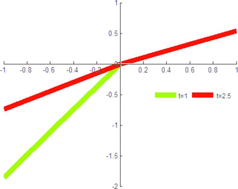But in the third quadrant, the prospect function with t=1 has distinct shape from that with t=2.5, moreover, the shape of the prospect function with t=1 is deeper. Thus, we can conclude when there is a loss, the larger the value of t is, the greater the partial dominance degree will be, and the flatter the shape of prospect function will become.

Furthermore, the ranking result is also varied with different values of t. To this end, we make further investigation on the final ranking order with the value of t varying from 0.025 to 25, as is outlined in Table 12.

t	Ranking Order
t=0.025	The USA ≻ China ≻ Canada ≻ Denmark ≻ Russia ≻ Norway
t=0.25	The USA ≻ China ≻ Canada ≻ Denmark ≻ Russia ≻ Norway
t=0.5	The USA ≻ China ≻ Canada ≻ Denmark ≻ Russia ≻ Norway
t=1	The USA ≻ China ≻ Canada ≻ Russia ≻ Denmark ≻ Norway
t=2	The USA ≻ China ≻ Canada ≻ Russia ≻ Denmark ≻ Norway
t=2.25	The USA ≻ China ≻ Canada ≻ Russia ≻ Denmark ≻ Norway
t=2.5	The USA ≻ China ≻ Canada ≻ Russia ≻ Denmark ≻ Norway
t=5	The USA ≻ China ≻ Russia ≻ Canada ≻ Denmark ≻ Norway
t=10	The USA ≻ Russia ≻ China ≻ Canada ≻ Denmark ≻ Norway
t=25	The USA ≻ Russia ≻ Canada ≻ China ≻ Denmark ≻ Norway

Table 12

The ranking order with different values of t.

From the results in Table 12, we can observe that the ranking order has slight changes as the value of t varies from 0.025 to 25. The best candidate is always the USA and the worst one is always Norway.

In theory, when t<1, the partial dominance degree has a reverse relationship with the value of t, namely, the loss is gradually strengthened with the value of t changing from 1 to 0, but when t≥1, the partial dominance degree has a positive relation with the value of t, that is, the loss is increasingly receded as the value of t increases. In this paper, this phenomenon is proved.

According to previous research results, the results are more reliable and convincing when the value of t is between 2 and 2.5. In this paper, the ranking order of six countries remains unaltered when the value of t varies from 2 to 2.5, indicating the robustness of the fuzzy TODIM method.

6. CONCLUSIONS

To overcome the drawbacks of PDHFSs, we extend single-valued occurring probability into interval-valued probability and propose the concept of IVPDHFSs. First, a series of IVPDHFSs are defined, such as generalized IVPDHFSs, ordered IVPDHFSs and normalized IVPDHFSs. We also give some operations and comparison method for IVPDHFEs. In addition, the ordered distance measure is defined to calculate the deviation of any two IVPDHFSs, the ordered similarity measure is also defined to derive the weight information of DMs. Moreover, to fuse the information provided by multiple DMs, the IVPDHFOWA operator is proposed. Based on the criteria weights derived from the water-filling theory- based model, a three-phased MCGDM framework is designed under IVPDHFSs circumstance. Finally, an example regarding Arctic risk evaluation is introduced to demonstrate the feasibility and acceptance of our three-phased MCGDM framework. The results of comparative analysis and sensitive analysis also show that the proposed three-phased MCGDM framework is reasonable and efficient.

In future research, we intend to investigate IVPDHFSs theory and apply more MCDM techniques to cope with practical problems within IVPDHFSs environment.

CONFLICT OF INTEREST

The authors declare no conflicts of interest.

AUTHORS' CONTRIBUTIONS

Peide Liu: Conceptualization, methodology, formal analysis, writing–writing–review and editing, supervision, funding acquisition.

Shufeng Cheng: Conceptualization, methodology, validation, investigation, writing–original draft preparation, visualization.

ACKNOWLEDGMENTS

This paper is supported by the National Natural Science Foundation of China (Nos. 71771140 and 71471172), 文化名家暨“四个一批”人才项目 (Project of cultural masters and “the four kinds of a batch” talents), the Special Funds of Taishan Scholars Project of Shandong Province (No. ts201511045), and Shandong Provincial Social Science Planning Project (Nos. 17BGLJ04, 16CGLJ31 and 16CKJJ27).

REFERENCES

1.P. Liu, F. Jin, X. Zhang, Y. Su, and M. Wang, Research on the multi-attribute decision-making under risk with interval probability based on prospect theory and the uncertain linguistic variables, Knowl. Based Syst., Vol. 24, 2011, pp. 554-561.

2.P. Liu, Y. Li, M. Zhang, L. Zhang, and J. Zhao, Multiple-attribute decision-making method based on hesitant fuzzy linguistic Muirhead mean aggregation operators, Soft Comput., Vol. 22, 2018, pp. 5513-5524.

3.P. Liu and F. Teng, Some Muirhead mean operators for probabilistic linguistic term sets and their applications to multiple attribute decision-making, Appl. Soft Comput., Vol. 68, 2018, pp. 396-431.

4.Z. Liu and P. Liu, Intuitionistic uncertain linguistic partitioned Bonferroni means and their application to multiple attribute decision-making, Int. J. Syst. Sci., Vol. 48, 2017, pp. 1092-1105.

5.G. Yu, W. Fei, and D. Li, A compromise-typed variable weight decision method for hybrid multiattribute decision making, IEEE Trans. Fuzzy Syst., Vol. 27, 2019, pp. 861-872.

6.L. Zadeh, Fuzzy sets, Inf. Control, Vol. 8, 1965, pp. 338-353.

7.S. Parsons, Current approaches to handling imperfect information in data and knowledge bases, IEEE Trans. Knowl. Data Eng., Vol. 8, 1996, pp. 353-372.

8.V. Torra, Hesitant fuzzy sets, Int. J. Intell. Syst., Vol. 25, 2010, pp. 529-539.

9.Z. Xu and M. Xia, Distance and similarity measures for hesitant fuzzy sets, Inf. Sci., Vol. 181, 2011, pp. 2128-2138.

10.B. Zhu, Z. Xu, and M. Xia, Hesitant fuzzy geometric Bonferroni means, Inf. Sci., Vol. 205, 2012, pp. 72-85.

11.Z. Zhang, Hesitant fuzzy power aggregation operators and their application to multiple attribute group decision making, Inf. Sci., Vol. 234, 2013, pp. 150-181.

12.R. Rodríguez, B. Bedregal, H. Bustince, Y. Dong, B. Farhadinia, C. Kahraman, et al., A position and perspective analysis of hesitant fuzzy sets on information fusion in decision making. Towards high quality progress, Inform. Fusion, Vol. 29, 2016, pp. 89-97.

13.G. Wei, Hesitant fuzzy prioritized operators and their application to multiple attribute decision making, Knowl. Based Syst., Vol. 31, 2012, pp. 176-182.

14.Z. Xu and X. Zhang, Hesitant fuzzy multi-attribute decision making based on TOPSIS with incomplete weight information, Knowl. Based Syst., Vol. 52, 2013, pp. 53-64.

15.R. RodríGuez, L. MartıNez, and F. Herrera, A group decision making model dealing with comparative linguistic expressions based on hesitant fuzzy linguistic term sets, Inf. Sci., Vol. 241, 2013, pp. 28-42.

16.R. Rodríguez, L. Martinez, and F. Herrera, Hesitant fuzzy linguistic term sets for decision making, IEEE Trans. Fuzzy Syst., Vol. 20, 2012, pp. 109-119.

17.N. Chen, Z. Xu, and M. Xia, Interval-valued hesitant preference relations and their applications to group decision making, Knowl. Based Syst., Vol. 37, 2013, pp. 528-540.

18.B. Farhadinia, Information measures for hesitant fuzzy sets and interval-valued hesitant fuzzy sets, Inf. Sci., Vol. 240, 2013, pp. 129-144.

19.J. Wang, J. Wu, J. Wang, H. Zhang, and X. Chen, Interval-valued hesitant fuzzy linguistic sets and their applications in multi-criteria decision-making problems, Inf. Sci., Vol. 288, 2014, pp. 55-72.

20.D. Joshi and S. Kumar, Interval-valued intuitionistic hesitant fuzzy Choquet integral based TOPSIS method for multi-criteria group decision making, Eur. J. Oper. Res., Vol. 248, 2016, pp. 183-191.

21.Z. Zhang, Interval-valued intuitionistic hesitant fuzzy aggregation operators and their application in group decision-making, J. Appl. Math., Vol. 2013, 2013. 33

22.B. Zhu, Z. Xu, and M. Xia, Dual hesitant fuzzy sets, J. Appl. Math., Vol. 2012, 2012. 13

23.G. Qian, H. Wang, and X. Feng, Generalized hesitant fuzzy sets and their application in decision support system, Knowl. Based. Syst., Vol. 37, 2013, pp. 357-365.

24.C. Wang, Q. Li, X. Zhou, and T. Yang, Hesitant triangular fuzzy information aggregation operators based on bonferroni means and their application to multiple attribute decision making, Sci. World J., Vol. 2014, 2014. 15

25.Z. Xu and W. Zhou, Consensus building with a group of decision makers under the hesitant probabilistic fuzzy environment, Fuzzy Optim. Decis. Mak., Vol. 16, 2017, pp. 481-503.

26.R. Krishankumar, K. Ravichandran, S. Kar, P. Gupta, and M. Mehlawat, Interval-valued probabilistic hesitant fuzzy set for multi-criteria group decision-making, Soft Comput., Vol. 23, 2019, pp. 10853-10879.

27.C. Song, H. Zhao, Z. Xu, and Z. Hao, Interval-valued probabilistic hesitant fuzzy set and its application in the Arctic geopolitical risk evaluation, Int. J. Intell. Syst., Vol. 34, 2019, pp. 627-651.

28.J. Ye, Correlation coefficient of dual hesitant fuzzy sets and its application to multiple attribute decision making, Appl. Math. Model., Vol. 38, 2014, pp. 659-666.

29.Z. Su, Z. Xu, H. Liu, and S. Liu, Distance and similarity measures for dual hesitant fuzzy sets and their applications in pattern recognition, J. Intell. Fuzzy Syst., Vol. 29, 2015, pp. 731-745.

30.L. Wang, Q. Shen, and L. Zhu, Dual hesitant fuzzy power aggregation operators based on Archimedean t-conorm and t-norm and their application to multiple attribute group decision making, Appl. Soft Comput., Vol. 38, 2016, pp. 23-50.

31.P. Singh, A new method for solving dual hesitant fuzzy assignment problems with restrictions based on similarity measure, Appl. Soft Comput., Vol. 24, 2014, pp. 559-571.

32.C. Wang, Q. Li, and X. Zhou, Multiple attribute decision making based on generalized aggregation operators under dual hesitant fuzzy environment, J. Appl. Math., Vol. 2014, 2014. 12

33.Z. Ren, Z. Xu, and H. Wang, Dual hesitant fuzzy VIKOR method for multi-criteria group decision making based on fuzzy measure and new comparison method, Inf. Sci., Vol. 388, 2017, pp. 1-16.

34.D. Yu and D. Li, Dual hesitant fuzzy multi-criteria decision making and its application to teaching quality assessment, J. Intell. Fuzzy Syst., Vol. 27, 2014, pp. 1679-1688.

35.D. Yu, D. Li, and J. Merigó, Dual hesitant fuzzy group decision making method and its application to supplier selection, Int. J. Mach. Learn. Cyb., Vol. 7, 2016, pp. 819-831.

36.N. Zhao, Z. Xu, and F. Liu, Group decision making with dual hesitant fuzzy preference relations, Cogn. Comput., Vol. 8, 2016, pp. 1119-1143.

37.Z. Ren and C. Wei, A multi-attribute decision-making method with prioritization relationship and dual hesitant fuzzy decision information, Int. J. Mach. Learn. Cyb., Vol. 8, 2017, pp. 755-763.

38.J. Merigó, Fuzzy decision making with immediate probabilities, Comput. Ind. Eng., Vol. 58, 2010, pp. 651-657.

39.G. Wei and J. Merigó, Methods for strategic decision-making problems with immediate probabilities in intuitionistic fuzzy setting, Sci. Iran., Vol. 19, 2012, pp. 1936-1946.

40.Z. Hao, Z. Xu, H. Zhao, and S. Zhan, Probabilistic dual hesitant fuzzy set and its application in risk evaluation, Knowl. Based Syst., Vol. 127, 2017, pp. 16-28.

41.W. Zeng, Y. Xi, Q. Yin, and P. Guo, Weighted dual hesitant fuzzy sets and its application in group decision making, IEEE, in 2018 14th International Conference on Computational Intelligence and Security (CIS) (Hangzhou), 2018, pp. 77-82.

42.M. Xia and Z. Xu, Hesitant fuzzy information aggregation in decision making, Int. J. Approx. Reason., Vol. 52, 2011, pp. 395-407.

43.P. Liu, S. Cheng, and Y. Zhang, An extended multi-criteria group decision-making PROMETHEE method based on probability multi-valued neutrosophic sets, Int. J. Fuzzy Syst., Vol. 21, 2019, pp. 388-406.

44.D. Palomar and J. Fonollosa, Practical algorithms for a family of waterfilling solutions, IEEE Trans. Signal Process., Vol. 53, 2005, pp. 686-695.

45.H. Zhao, A. Yan, and P. Wang, On improving reliability of case-based reasoning classifier, Acta Automatica Sinica, Vol. 40, 2014, pp. 2029-2036. http://en.cnki.com.cn/Article_en/CJFDTotal-MOTO201409024.htm

46.X. Liu, Z. Wang, and S. Zhang, A new methodology for hesitant fuzzy emergency decision making with unknown weight information, Complexity, Vol. 2018, 2018. 12

47.H. Wang, X. Zhao, and G. Wei, Dual hesitant fuzzy aggregation operators in multiple attribute decision making, J. Intell. Fuzzy Syst., Vol. 26, 2014, pp. 2281-2290.

<Previous Article In Issue

Download article (PDF)

Next Article In Issue>

Journal: International Journal of Computational Intelligence Systems
Volume-Issue: 12 - 2
Pages: 1393 - 1411
Publication Date: 2019/12/06
ISSN (Online): 1875-6883
ISSN (Print): 1875-6891
DOI: 10.2991/ijcis.d.191119.001 How to use a DOI?
Open Access: This is an open access article distributed under the CC BY-NC 4.0 license (http://creativecommons.org/licenses/by-nc/4.0/).

Cite this article

ris enw bib

TY  - JOUR
AU  - Peide Liu
AU  - Shufeng Cheng
PY  - 2019
DA  - 2019/12/06
TI  - Interval-Valued Probabilistic Dual Hesitant Fuzzy Sets for Multi-Criteria Group Decision-Making
JO  - International Journal of Computational Intelligence Systems
SP  - 1393
EP  - 1411
VL  - 12
IS  - 2
SN  - 1875-6883
UR  - https://doi.org/10.2991/ijcis.d.191119.001
DO  - 10.2991/ijcis.d.191119.001
ID  - Liu2019
ER  -

download .riscopy to clipboard

	c1(MC)	c2(DD)	c3(EI)	c4(MR)
The USA	⟨{0.7\|0.2,0.6\|0.2,0.5\|0.6},{0.2\|1}⟩	〈0.7\|1,0.25\|1〉	〈0.2\|1,0.2\|1〉	〈0.7\|0.5,0.6\|0.5,0.3\|1〉
Canada	〈0.1\|1,0.4\|1〉	〈0.3\|1,0.7\|1〉	〈0.7\|1,0.3\|0.5,0.2\|0.5〉	〈0.3\|1,0.3\|1〉
Russia	〈0.6\|1,0.35\|1〉	〈0.56\|1,0.2\|1〉	〈0.1\|1,0.7\|1〉	〈0.2\|0.6,0.4\|0.4,0.4\|1〉
Denmark	〈0.05\|0.7,0.2\|0.3,0.5\|1〉	⟨{0.3\|0.5,0.2\|0.5},{0.6\|0.5,0.5\|0.5}⟩	〈0.8\|1,0.15\|1〉	〈0.2\|1,0.6\|1〉
China	〈0.15\|1,0.8\|1〉	〈0.5\|1,0.5\|1〉	〈0.8\|0.6,0.6\|0.4,0.15\|1〉	〈0.2\|1,0.7\|0.9,0.6\|0.1〉
Norway	〈0.08\|1,0.6\|1〉	〈0.1\|0.6,0.3\|0.4,0.7\|1〉	〈0.3\|1,0.65\|1〉	〈0.5\|1,0.2\|0.3,0.4\|0.7〉

	c1(MC)	c2(DD)	c3(EI)	c4(MR)
The USA	〈0.5\|1,0.5\|1〉	〈0.2\|1,0.4\|0.8,0.6\|0.2〉	⟨{0.7\|0.4,0.4\|0.6},{0.3\|0.7,0.2\|0.3}⟩	〈0.6\|0.7,0.7\|0.3,0.25\|1〉
Canada	〈0.3\|0.5,0.5\|0.5,0.4\|1〉	〈0.1\|10.6\|0.6,0.8\|0.4〉	⟨{0.4\|0.8,0.3\|0.2},{0.5\|0.3,0.4\|0.7}⟩	〈0.2\|0.3,0.3\|0.7,0.6\|1〉
Russia	〈0.1\|0.1,0.2\|0.9,0.5\|1〉	⟨{0.3\|0.5,0.2\|0.5},{0.3\|0.5,0.2\|0.5}⟩	〈0.2\|1,0.7\|0.6,0.5\|0.4〉	〈0.5\|1,0.4\|1〉
Denmark	〈0.2\|1,0.7\|0.1,0.6\|0.9〉	〈0.1\|1,0.7\|1〉	〈0.2\|1,0.6\|1〉	〈0.2\|0.8,0.1\|0.2,0.3\|0.4,0.2\|0.6〉
China	〈0.2\|1,0.7\|1〉	〈0.45\|1,0.5\|1〉	〈0.8\|0.9,0.6\|0.1,0.11\|1〉	〈0.3\|1,0.2\|1〉
Norway	〈0.4\|0.4,0.5\|0.6,0.5\|1〉	〈0.3\|0.4,0.4\|0.6,0.7\|1〉	〈0.3\|1,0.6\|1〉	〈0.2\|1,0.6\|1〉

	c1(MC)	c2(DD)	c3(EI)	c4(MR)
The USA	〈0.4\|1,0.5\|1〉	〈0.9\|1,0.1\|1〉	〈0.3\|1,0.5\|0.4,0.6\|0.6〉	〈0.6\|1,0.3\|1〉
Canada	〈0.75\|1,0.2\|1〉	〈0.4\|1,0.6\|1〉	〈0.2\|0.7,0.4\|0.3,0.2\|1〉	〈0.3\|1,0.6\|1〉
Russia	〈0.6\|0.6,0.8\|0.4,0.1\|1〉	〈0.5\|1,0.2\|1〉	〈0.1\|1,0.8\|1〉	〈0.2\|0.7,0.4\|0.3,0.6\|1〉
Denmark	〈0.2\|1,0.7\|1〉	〈0.5\|0.6,0.7\|0.4,0.1\|1〉	⟨{0.3\|0.3,0.5\|0.7},{0.2\|0.5,0.5\|0.5}⟩	〈0.1\|0.6,0.3\|0.4,0.6\|1〉
China	⟨{0.3\|0.7,0.4\|0.3},{0.4\|0.6,0.5\|0.4}⟩	〈0.6\|1,0.2\|0.5,0.1\|0.5〉	〈0.7\|1,0.2\|1〉	⟨{0.1\|0.45,0.3\|0.55},{0.5\|0.5,0.65\|0.5}⟩
Norway	〈0.2\|0.2,0.1\|0.8,0.7\|1〉	〈0.2\|1,0.8\|1〉	〈0.2\|0.8,0.3\|0.2,0.6\|1〉	〈0.35\|1,0.5\|0.5,0.6\|0.5〉