
Artificial Neural Network to Model Managerial Timing Decision: Non-linear Evidence of Deviation from Target Leverage
- DOI
- 10.2991/ijcis.d.191101.002How to use a DOI?
- Keywords
- Capital structure; Market timing; Multiple regression model; Artificial neural network
- Abstract
The current study highlights the utilization of a non-linear model to analyze an important decision-making process in the study of corporate finance where managers are deciding on the capital structure of a firm. This study compares the results from based on the unbalanced panel data multiple regression for firm fixed effects relative to the artificial neural networks, i.e., ANN, with known determinants of capital structure as control variables for a sample of UK firms respectively. Results of the study show that firms are timing away from target levels which challenges the current findings in the literature. The ANN model achieves a better fit based on the root of mean-squared error (RMSE) values which provides a more accurate forecast. Thus, the nature of balancing between cost of being off-target versus benefits gained from timing the equity market is non-linear and which is captured by ANN. Implications from the study allow market players to understand the process of achieving optimal capital structure to maximize firm value and thus benefit all stakeholders.
- Copyright
- © 2019 The Authors. Published by Atlantis Press SARL.
- Open Access
- This is an open access article distributed under the CC BY-NC 4.0 license (http://creativecommons.org/licenses/by-nc/4.0/).
1. INTRODUCTION
The current study examines the behavior of firms in timing the equity market based on the mispricing criteria based on a sample of UK firms in order to evaluate its impact on capital structure which consequently affects firm value. The theoretical expectation of managers timing the equity market predicts that managers would opt for equity issues during periods of overvaluation and lean toward debt during periods of undervaluation.
The need for the study arises from the impact of financing choices on firm value which is derived from the sum of present value of future cash flows from all projects in the firm. Financing patterns influences the cost of capital which in turn leads to changes in the present value despite future cash flows remaining constant. This is especially of concern to managers given that firm value is a direct reflection of shareholders wealth where the ultimate aim of corporate managers is to maximize shareholders' wealth [1]. Therefore, the current study investigates the impact of changes in equity prices which is an exogenous factor relative to managerial decision-making in issuing securities in order to operate at optimal or target levels of leverage where firm value is maximized [2,3]. It further aims to providing insights into the motives for managerial decision-making which impact stakeholders as a whole given that investment decisions at the firm level are part and parcel of the aggregate investment function which is dependent on borrowings [4].
In addition, the current study incorporates targeting behavior into timing attempts by managers. The expectation for the study is derived from the literature where firms are found to have target ratios yet actively time the equity market [5,6]. The literature further shows that the incentive to time the equity market is driven by the extent of deviation from target leverage [7,8]. Given the findings in the literature, we provide an alternative explanation of the model where firms are timing away from target levels rather than toward target levels. To the best of our knowledge, this is the first study to illustrate the non-linear impact which leads to firms moving away from target level rather than toward target levels. The model utilized in this study considers the extent firms deviate from target levels and the influence of equity mispricing on the extent of deviation.
The literature in studies concerning capital structure are rich and provide many aspects of contention in the literature on the impact of equity mispricing on capital structure decisions [9]. However, the ability of the model to predict has been rarely tested [10]. Given the need for analysis of capital structure determinants to be relevant to the empirical data, predictive ability is useful for managerial decision-making as the literature indicates mixed results on the impact of leverage on firm value [11,12]. In addition, the value of a firm has been proven to be highly dependent on operating at optimal levels as well as equity market timing decisions by managers which impact decision-making [13]. However, the opposing situation is also evidenced in the literature where firms issuing during times of high equity valuations are driven by intentions to invest in real assets [14]. Thus, the findings from predictive model would also allow improved inferences to decision-making at investor and managerial levels.
Thus, this study employs artificial neural network (ANN) to predict firms' deviation from target capital structure as a consequence of equity mispricing given that ANN is able to provide solutions for forecast problems [15–18]. The approach for utilizing ANN provides the model the ability to establish relationships between equity mispricing (the variable of concern) and the deviation from target levels rather than specifying the nature of the relationship from the onset of the analysis.
Furthermore, ANN does not require the assumption that about distribution of the equity prices before the analysis. Assumptions on the pre-set of the analysis creates a biasness in the results given that most studies find that equity prices behave in random manner and thus are difficult to predict [19]. Employing analysis by assuming normality of distribution of equity prices would thus lead to flawed analysis and results as prices tend to be based on random walk patterns [20]. Thus, the predictive ability of the ANN model employed provides intelligent learning capabilities which are based on training data, i.e., historical data which improves the decision-making at the managerial level given that the analysis takes into consideration the random nature of equity prices.
The approach is particular of interest to the analyze firms' timing behavior given the inputs tend to be correlated (market and book measures of financial variables) and it is likely that targeting behavior is non-linear as predicted by the dynamic capital structure [21].
The study is thus aimed at answering two quantitatively themed questions in order to provide a qualitative opinion on the impact of timing attempts by managers on deviation from leverage levels as well as firm value: whether equity mispricing leads to deviation from target leverage; does the non-linear approach utilized in the current study provide an improve model fitting and ability to forecast timing attempt by managers.
The rest of the paper is organized as follows: Section 2 provides the literature review to motivate the study. Section 3 describes the data source, the variables and methodology. Section 4 compares the results from the linear multiple regression and ANN and explanation on the outcomes. Section 5 summarizes the findings and concludes the paper.
2. REVIEW OF THE RELEVANT LITERATURE
There have been various studies concerning the trade-off theory of capital structure where firms are regularly trading-off the cost and benefit of debt financing in order to reach target levels. Managers attempt to maximize firm value and hence are interested in reaching the target level where capital structure is optimal and cost of capital is minimized [22]. Despite this, firms are unable to operate at optimal levels. This deviation from target levels arise due to market imperfections which are attributed to transaction costs as well as information asymmetry. Thus, firms tend to temporarily deviating from optimal levels [23].
The aim to reach target level is evidenced from survey studies in the literature where managers do indeed issue securities with a target in mind [24–26]. Timing attempts are also shown to be a primary drive for decision-making in security issues [27–30].
The trade-off theory of capital structure predicts that firms have an optimal level of leverage that managers aims to reach in order to maximize firm value. Thus, managers are constantly trading-off the benefits of debt capital with the potential associated costs such as potential bankruptcy costs [31]. Equilibrium is reached at a point when additional borrowing would reduce firm value [32]. The empirical literature provides ample proof of firms target adjustment behavior based on the partial adjustment model approach which points toward a non-linear model to explain changes in capital structure [33–35]. In addition, firms are found to offset deviation from earnings and losses via securities issues [36,37]. Furthermore, it is found that dynamic models indicate that adjustment costs are existent when estimating target adjustment behavior based on the dynamic duration approach [38,39].
The literature suggests that firms could indeed deviate from optimal levels due to individual managers having a pre-set target level and yet also be interested in timing security issues, hence tend to allow leverage levels tend to have a band or acceptable range rather than a hard target ratio [40,41]. Furthermore, given that equity issues tend to be costly, managers have the incentive to clump issues to raise large levels of financing which then allows managers the ability to time equity markets [13,42]. This issue is further compounded for firms with greater levels of information asymmetry and thus create an incentive for managers to prefer debt issues given that equity prices are suppressed and thus leading to exceeding target levels. In the event of equity prices recover, then these managers would have further incentive to issue even greater levels of equity in anticipation of difficulty of raising further equity in the future to potential undervaluation. Thus, managers are also keen to build financial slack where there is a market-oriented trade-off.
In addition, firms are able to deviate from target levels given that the cost of deviation from target levels arising from equity issues tend to be small and transitory in nature [5,43]. Arguably, firms are also found to be pursuing equity market timing strategy for in the short-run yet reverting to optimal levels in the long-run [28,44,45]. In addition, firms' deviation from target levels is also influence by its sensitivity to its cost of equity capital where firms with higher cost of equity tend to adjust to target levels at more rapid rates [46].
Firms ability to time the equity market also influences its future growth given that timed issues tend to yield in greater levels of cash and thus providing opportunity for further growth [2]. The potential economic gains are further evidenced in the literature where via open market repurchase of outstanding shares. Firms with undervalued equity as well as operating at leverage levels which are below target levels tend to gain the most from repurchase programs as evidenced in gains in share prices [8]. Furthermore, empirical findings further indicate that firms are able to reach optimal levels faster based equity mispricing [7].
Recent studies further indicate that firms deviate from target leverage regularly and the ability to adjust is a function of its cost of equity which is linked to exogenous factors including risk premiums and adjustment costs [46]. Thus, firms with greater levels of variability in changes of equity costs linked to deviation from optimal levels tend to adjust faster leading to an asymmetry in response [45]. In addition, the literature further documents that shareholders are not in favor of reduction in leverage despite it reducing firm value creating a ratchet effect where firms tend to operate at sub-optimal levels [47]. Further contention is found where direct measures of adjustment costs are found to be positively related to rate of adjustment rather than the expected negative [43]. The nature of the relationship between the theoretical and empirical findings are puzzling. These findings in the literature validate the need to evaluate the deviation from target levels from a non-linear point of view which supports the analysis in this study based on the ANN approach incorporating latent variables which are unobservable to provide predictive power.
In addition, the predictive relationship provided by the model allows the analysis to capture the underlying relationships within the dataset of the selected sample [48]. Current studies also utilize linear models which are not able to capture the distinction between deviation from target leverage levels relative to adjustment to target levels to reach optimal points. This is a result of the model selection which fails to recognize the relationship between and within determinants variables [49]. Selection of linear models to examine issues in corporate finance also lacks the ability to distinguish random noise from the non-linear relationship which is lumped into the error term [50].
The application of the ANN model in this study is thus based on the ability of the model to select data which is important via distillation in the hidden layer which allows for a more accurate estimation of the parameters for evaluating the impact of timing equity issues on deviation from target leverage [51]. Thus, data which is redundant is left out of the analysis hence improving the accuracy of the results in order to identify the impact of equity mispricing, an exogenous variable on the complex decision-making process at firm level [52].
3. SAMPLE AND METHODOLOGY
3.1. Data Selection
The data in this study is extracted from the Datastream database for all UK firms for the period of 1991–2018. The sample includes inactive firms in order to mitigate potential problems arising from selection and survivor bias. Financial firms are excluded from the sample. In order to account for heterogeneity arising from industry effects, we include classify firms into 15 different industries which leads to the inclusion of 14 industry dummies in the analysis. Industry classifications are thus provided in Appendix. Definition of variables are presented in Table 1 below.
| Variable | Definition |
|---|---|
| Book debt (BD) | Book debt scaled by total assets |
| Market debt (MD) | Book debt scaled by market value of equity plus book value of debt |
| Non-debt tax shield (NDTS) | The ratio of depreciation expenses scaled by total assets |
| Firm size (SIZE) | Natural logarithm of total assets in millions of 1991 pounds |
| Asset Tangibility [TANG] | Net property, plant and equipment divided by total assets |
| Effective tax rate (ETR) | Total tax divided by total taxable income |
| Industry leverage (INDL) | Median of the leverage level of the industry |
Definition of variables utilized in the study
In order to control for the impact of outliers, we winsorize the sample by 1% on either end of the distribution for all variables. Missing observations are automatically excluded. The final sample consists of 14,436 firm-year observations. Mean values of the sample is presented with standard deviation in parenthesis in Table 2 below.
| 1 | 2 | 3 | 4 | 5 | 6 | 7 | |
|---|---|---|---|---|---|---|---|
| Pre-issue debt | 0.1825 | 0.1836 | 0.1802 | 0.1233 | 0.3422 | 0.1452 | 0.2956 |
| (0.1638) | (0.1536) | (0.1599) | (0.1622) | (0.1620) | (0.1529) | (0.1925) | |
| Post-issue debt | 0.1896 | 0.2891 | 0.3038 | 0.0825 | 0.1828 | 0.1581 | 0.2019 |
| (0.1596) | (0.1028) | (0.1245) | (0.1299) | (0.1861) | (0.1520) | (0.1825) | |
| Net debt issued | 0.0156 | 0.1405 | 0.1822 | 0.0006 | −0.2015 | 0.0001 | −0.1325 |
| (0.1192) | (0.0825) | (0.1256) | (0.0199) | (0.1520) | (0.0195) | (0.1140) | |
| Net equity issued | 0.0568 | 0.0005 | −0.1860 | 0.2855 | 0.2625 | −0.1428 | −0.0005 |
| (0.1962) | (0.0828) | (0.1472) | (0.2522) | (0.2204) | (0.1253) | (0.0192) | |
| NDTS | 0.0295 | 0.0299 | 0.0325 | 0.0282 | 0.0305 | 0.0300 | 0.0318 |
| (0.3866) | (0.3869) | (0.2485) | (0.3625) | (0.3204) | (0.2825) | (0.3922) | |
| SIZE | 14.8824 | 15.2236 | 15.3608 | 14.0623 | 13.9528 | 15.2562 | 14.8920 |
| (2.4692) | (2.3691) | (2.2899) | (2.2104) | (2.1922) | (2.3082) | (2.5204) | |
| TANG | 0.3528 | 0.4088 | 0.3891 | 0.2401 | 0.3086 | 0.3506 | 0.3562 |
| (0.2208) | (0.2019) | (0.1822) | (0.1920) | (0.2138) | (0.2196) | (0.2196) | |
| ETR | 0.3063 | 0.2861 | 0.3951 | 0.1692 | 0.1526 | 0.3627 | 0.2199 |
| (1.0892) | (1.1025) | (0.8822) | (1.1022) | (1.0625) | (0.9652) | (0.9985) | |
| Equity undervalued | 48.82% | 72.35% | 81.36% | 18.26% | 2.96% | 62.48% | 19.92% |
| Observations | 14,436 | 1,968 | 484 | 1,690 | 590 | 869 | 1,268 |
1- All firms, 2- Pure Debt Issuers, 3- Issue Debt and Repurchase Equity, 4- Pure Equity Issuers, 5- Issue Equity and Retire Debt, 6- Pure Equity Repurchases, 7- Pure Debt Reductions
NDTS, non-debt tax shield; SIZE, firm size; TANG, asset tangibility; ETR, effective tax rate.
Descriptive statistics of the sample
The figures presented in Table 2 indicate that firm leverage is stationary in pre-issue and post-issue stage. Interestingly, pure debt issuers tend to have equity which is undervalued about 70% of the time. In addition, firms which issue debt and repurchase equity tend to have equities which are undervalued about 80% of the time. The overall average of debt levels which is found to be 18% in the sample does provide an interesting observation which further validates the main notion of the study where firms are not attempting to reduce deviation from target levels (assuming that the target levels is close to the overall average level). In both instances, firms are inclined to increase debt levels which leads to deviation from target levels. Furthermore, these firms than to have profitability levels which are greater than the sample average. Both categories of firms also tend to pursue a low cash holding strategy which further validates a greater inclination of debt issues.
Analyzing pure equity issues show that equities tend to be overvalued 82% of the time. In addition, these firms' action of issuing equity during periods of overvaluation does not seem to bring them closer to the overall sample average. In fact, it does indicate that equity overvaluation tends to push firms away from target levels. However, a contrary pattern is observed for firms that go for equity issues whilst opting to reduce debt levels via redemption of borrowings where the intention seems to be driven targeting behavior. Pure equity issues tend to have greater levels of cash holdings. Firms which opt for pure equity repurchase on the other hand are driven by timing motives rather than targeting behavior where whilst equities tend to be undervalued, pre- and post-issues of leverage do not change significantly. Firms which opt for pure reduction of debt levels on the other hand tend to be driven by balancing capital structure where equity tends to be overvalued 84% of the time leading to mechanical reduction in market leverage ratios [53].
3.2. Equity Mispricing
In order to estimate the intrinsic value of equities and hence derive the mispricing element by the market, the study utilizes the residual income model which is derived mainly from the accounting literature [54,55]. The literature documents that the model is able to predict share repurchase activities by firms, valuation for mergers and acquisitions as well as predicting returns for shares in international markets [56–58].
The current study adopts the approach of decomposing the book-to-market ratio into 2 components which are the ratio of book value to intrinsic value times the ratio of intrinsic value to market value [59]. The first component captures the value to price (VP ratio) which is a direct measure of mispricing as evidenced in the literature and is able to predict market timing attempts by managers [60,61].
The purpose of adoption of the decomposition instead of the market-to-book ratio for measuring equity mispricing is given that the literature documents that the ratio is unable to predict timing attempts by managers [2,62]. This can be attributed due to the measure capturing growth options as well as mispricing and due to inconsistency in relationships over the long-run and tends to be time dependent [7,63].
The residual income model estimates firms' equity value based on the discounted expected earnings which exceeds expectations on the returns derived from book value. This approach is similar to the economic value-added approach (EVA). The model is thus measuring firm value (V0) as
In equilibrium, the MISP ratio would be equal to 1. A value of greater than 1 implies undervaluation whilst a value of greater than 1 implies overvaluation.
3.3. Multiple Regression Model
In order to measure the deviation from target levels, we employ a two-stage model which as described as follows:
The estimation from Equation (4) is based on the debt ratio at time t+1 based on the literature which measures the desired debt ratio rather than the historical debt ratio [62]. The model captures known determinants as Witα which acts as control variables based on the empirical priors discussed above. The 2-stage model captures the deviation from target leverage level is calculated based on the difference between simulated values from Equation (4) above (D*t+1) versus the actual debt ratios (Dt+1). Thus, the second stage model is expressed as follows:
The key explanatory variable of concern to this study is the UNDVDit which takes the value of 1 when firms' equity is undervalued and 0 otherwise. Two additional control variables are incorporated into the model in order to capture the target adjustment behavior which allows us to isolate the impact of equity mispricing on deviation from target leverage. Dhi and Dlo take the values of one (or zero otherwise) if firms' borrowing levels in the previous year was in the top (bottom) fifth of the distribution accordingly [67].
3.4. Artificial Neural NetworkANN Model
The current study employs the back-propagation (BP) based on the neural network which consists of three distinctive layers: input, hidden and output [68,69]. The hidden layers allow the model to capture the non-linear effect in between the relationship of the variables. Each layer is connected to the next layer based on the connection between the multiple neurons. The interaction is complex which allows the model to capture the timing phenomenon being studied [17,70].
The approach utilized in this study is by allowing the historical firm-year data set act as a training mechanism for the neural network which will allow the estimations to capture the characteristics of the data set. Forecast errors are minimized by iteratively adjusting the model parameters based on the weights between the connections and node biased. In each training process, the input vector is selected to act as an input variable for the network. Based on this, the output of each processing unit was then propagated forward through the three layers in the network [71,72]. Figure 1 below illustrates the neural network utilized.
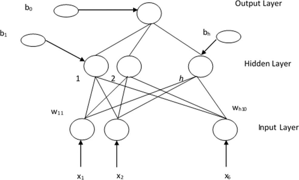
Model applied for neural network.
The input layer has six input variables. The hidden layer has h number of nodes whilst the output layer has a single note. In the training process, the network is presented with n pairs of input vectors which is matched to the corresponding output (X(1), y(1)), (X(2), y(2)), ⋯.., (X(n), y(n)). The inputs are based on a weighted sum and is expressed as follows:
4. EMPIRICAL RESULTS AND DISCUSSIONS
The results for estimating the target leverage at t+1 for both book and market leverage based on Equation (4) are reported in Table 3 below.
| Static |
Dynamic |
|||
|---|---|---|---|---|
| BD | MD | BD | MD | |
| NDTS | 0.2568*** | 0.2109*** | 0.1825*** | 0.1529*** |
| (0.0385) | (0.0520) | (0.0296) | (0.0191) | |
| SIZE | 0.0208*** | 0.0235*** | 0.0199*** | 0.0215*** |
| (0.0009) | (0.0012) | (0.0006) | (0.0011) | |
| TANG | 0.1236*** | 0.1402*** | 0.1195*** | 0.1385*** |
| (0.0208) | (0.0226) | (0.0192) | (0.0226) | |
| ETR | −0.0158*** | −0.205*** | −0.0144*** | −0.0184*** |
| (0.0025) | (0.0036) | (0.0012) | (0.0018) | |
| INDL | 0.5925*** | 0.7822*** | 0.4262*** | 0.5326*** |
| (0.0825) | (0.1826) | (0.0618) | (0.0819) | |
| Lagged dependent | – | – | 0.4896*** | 0.5622*** |
| – | – | (0.0256) | (0.0488) | |
| F-Test (p-values) | 0.00 | 0.00 | – | – |
| Average R2 | 0.1596 | 0.2488 | – | – |
| Adjusted R2 | – | – | 0.4695 | 0.5825 |
| AR (1) | – | – | −4.0825*** | −4.2506*** |
| AR (2) | – | – | 0.6925 | 0.7235 |
| Wald test (p-values) | – | – | 0.00 | 0.00 |
| Sargan test (p-values) | – | – | 0.28 | 0.33 |
| Observations | 14,436 | |||
| Period | 1991–2018 | |||
Significance level: *, ** and *** for 10%, 5% and 1% level, respectively. Standard errors are reported in parenthesis.
BD, book debt; MD, market debt; NDTS, non-debt tax shield; SIZE, firm size; TANG, asset tangibility; ETR, effective tax rate, INDL, industry leverage.
Estimating target leverage(t+1)
Target leverage levels are estimated based on the dynamic (2-step system GMM) as well as the static method [76,77]. The dynamic model is applied in this study together with the static model as an additional measure of robustness given that static model tend to have several limitations which include heterogeneity and endogeneity concerns [21,78]. In addition, the dynamic model allows the observation of firms' adjustment to target levels which validates the main objective of this study concerning the deviation from optimal levels. The lagged dependent is significant indicating that firms to indeed adjust to target levels. Furthermore, diagnostics of the model confirm the validity of the instruments based on the positive figure observed for AR(1) as well as the negative figure observed for AR (2) [79]. The Sargan test also fails to reject the null hypothesis further providing validation of the results whilst confirming firms do indeed adjust to target levels. The justification for using both the static and dynamic method is as an additional measure of robustness [7].
The standard errors on the dynamic model are corrected based on finite sample bias approach [80]. The main results are within our expectations where the non-debt tax shield has a positive relationship with target leverage levels [81,82]. This can be argued based on the view that firms with greater levels of fixed assets tend to have greater depreciation expenses and thus act as tax credits which provides greater levels of collateral when securing against debt issues. This leads to such firms being able to have greater levels of debt capacity [83]. The results also indicate that firms' size positively influences target leverage given that larger firms tend to have greater levels of diversification which reduces the volatility of their cash flows hence increasing their ability to service interest payments [84]. Reduction in the volatility of cash flows further reduces the potential for bankruptcy hence allowing firms to utilize the tax shield afforded by debt issues [85,86].
Asset tangibility is found to also have a positive relationship which is expected given that these assets are able to act as collateral and hence provide greater debt capacity [87]. The results also reveal a puzzling relationship between the effective tax rate and target levels which is negative and insignificant (Hang et al., 2018 [88] observe a similar relationship). Industry leverage levels tend to influence target levels where the variable is positive and significant [89].
4.1. Deviation from Target Leverage: Multiple Regression versus ANN
This section reports the results from the fitted values based on the simulated results obtained in Table 3 above to derive target leverage at t+1. The difference is then modeled based on Equation (5) and reported in Table 4 below. Columns 1 and 3 report the static and dynamic results based on the linear regression model for firm fixed effects which allow for clustering at firm and year level [90]. This gives improved results relative to clustering based on year or firm alone [91]. The results indicate that the MISP variable is insignificant. In addition, the VIF exceeds 20 indicating the problem of multi-collinearity. Furthermore, the root MSE for both the static and dynamic framework were relatively high.
| Static |
Dynamic |
ANN Sensitivity |
||||
|---|---|---|---|---|---|---|
| BD | MD | BD | MD | BD | MD | |
| UNDVD | −0.3625*** | −0.4299*** | −0.4695*** | −0.5025*** | −2.28 | −2.56 |
| (0.0638) | (0.0695) | (0.0722) | (0.0816) | – | – | |
| VIF | 36.45 | 38.96 | 29.95 | 32.44 | – | – |
| RMSE out-of sample | 0.82 | 0.84 | 0.85 | 0.88 | – | – |
| RMSE of training sample | – | – | – | – | 0.051 | 0.062 |
| RMSE of testing sample | – | – | – | – | 0.069 | 0.073 |
| Control variables | Yes | Yes | Yes | Yes | Yes | Yes |
| Adjusted R2 | 0.3925 | 0.4208 | 0.4899 | 0.6025 | – | – |
| Wald t (p-values) | 0.00 | 0.00 | 0.00 | 0.00 | – | – |
| Observations | 14,436 | |||||
| Period | 1991–2018 | |||||
Significance level: *, ** and *** for 10%, 5% and 1% level, respectively. Standard errors are reported in parenthesis.
ANN, artificial neural network; BD, book debt; MD, market debt; RMSE, root mean-squared error.
Comparing the impact of equity mispricing on deviation to target leverage: Multiple regression versus ANN sensitivity analysis
In order to resolve the problems above, the neural network sensitivity model is employed. Data during the period of 1991–2017 acts as a training data whilst data form the last year (2018) serves as the testing data. The BP approach with the (6-8-1) framework is utilized based on Equation (11). The results are reported in columns 2 and 4 of Table 4 above. Based on the results presented, it is found that the ANN model provides the lowest RMSE for in-sample and out-of-sample forecasting. Thus, the non-linear approach based on the ANN adoption allows the capture of sophisticated relationships among dependent and independent variable whilst integrating the impact of equity mispricing under the static and dynamic framework for target capital structure.
The results indicate that the relationship between equity mispricing and deviation from target leverage to be non-linear. In addition, the sign of the relative sensitivity of the ANN model resembles the sign of the coefficients in the regression model. Results indicate that the equity mispricing is the most important determinant when estimating the deviation from target leverage by priority based on the sensitivity from the ANN results.
The results provide interesting insights into the literature of corporate finance given the ongoing contention regarding the validity of the market timing theory to explain capital structure decisions [92,93]. Given that the MISP measure is the most important variable in explaining the rationale for deviating from target levels, it is an indication that managers timing attempts are deliberate and insiders being acutely aware of market prices departing from intrinsic value. In addition, it also paints managerial decision-making in a more realistic manner where managers are consistently weighing benefits of timing the equity market versus the costs of deviating from target levels. To some extent it also highlights the limitations of traditional linear regression models in capturing this effect.
The results are based on the assumption that firms are operating at optimal levels, i.e., they do not deviate from target leverage levels. However, this is an impractical assumption and thus the estimations would tend to suffer from endogeneity issues. In order to address the concerns, the first difference of the variable is thus taken where the following model is estimated:
Similar to the empirical approach above the undervaluation dummy is intended to capture the timing behavior. The results for regressing the model from Equation (11) is reported in Table 5 below.
| Static |
Dynamic |
ANN Sensitivity |
||||
|---|---|---|---|---|---|---|
| BD | MD | BD | MD | BD | MD | |
| UNDVD | −0.4896*** | −0.5344*** | −0.5625*** | −0.6204*** | −2.95 | −3.26 |
| (0.0812) | (0.0916) | (0.0925) | (0.1028) | – | – | |
| VIF | 42.44 | 45.68 | 33.42 | 36.42 | – | – |
| RMSE out-of sample | 0.85 | 0.88 | 0.89 | 0.91 | – | – |
| RMSE of training sample | – | – | – | – | 0.042 | 0.058 |
| RMSE of testing sample | – | – | – | – | 0.044 | 0.064 |
| Control variables | Yes | Yes | Yes | Yes | Yes | Yes |
| Adjusted R2 | 0.4205 | 0.4892 | 0.5622 | 0.6308 | – | – |
| Wald test (p-values) | 0.00 | 0.00 | 0.00 | 0.00 | – | – |
| Observations | 14,436 | |||||
| Period | 1991–2018 | |||||
Significance level: *, ** and *** for 10%, 5% and 1% level, respectively. Standard errors are reported in parenthesis.
ANN, artificial neural network; BD, book debt; MD, market debt; RMSE, root mean-squared error.
Comparison of results: Accounting for endogeneity concerns
The results indicate a similar pattern where the ANN model outperforms the linear regression model. In addition, undervaluation dummy is the most important variable in predicting the reason for deviation from target leverage levels. The results provide an indication where managers are constantly issuing debt during periods of undervaluation and issuing equity during periods of overvaluation. Thus, during periods of undervaluation, the distance and change in distance would be decreasing suggesting that firms are likely to be over target levels.
4.2. Accounting for Under- and Over-Levered Firms
In order to ensure that our results are robust and are able to cater for all firms regardless of their position relative to the target leverage levels, we further segregate the sample based on whether a firm is over or under the target leverage levels. The segregation allows inference of better insights from the analysis given that it provides a specific explanation for firms timing behavior whilst accounting for target adjustment behavior [7].
The rationale for distinguishing firms based current level of leverage being over or under optimal level arises from the expected rate of adjustment to target based on the corresponding cost of adjustment [86]. In addition, theoretical expectations which are validated by empirical findings indicate that firms above target levels would face greater pressures to adjust to target levels [94]. Furthermore, the interaction between equity mispricing and deviation from target levels may also differ given that firms which are above (below) target levels and have equities which are overvalued (undervalued) tend to adjust at more rapid rates [7].
In order to ensure the nature of the regression is consistent, we measure deviation as an absolute measure. The results for regressing Equations (5) and (12) are reported for in Table 6 below for over-levered firms. Results observed in Table 6 indicate that firms are likely to increase reliance on debt as a source of capital when equity prices are depressed. This would lead to the deviation from target leverage levels as observed in the significant coefficient. The ANN results further indicate that the dummy variable is the most important variable when predicting the extent of deviation from target leverage. The results are more evident when measuring change in deviation given that the first four columns are assuming that firms are operating at the optimal point.
| Static |
Dynamic |
ANN Sensitivity |
||||
|---|---|---|---|---|---|---|
| BD | MD | BD | MD | BD | MD | |
| UNDVD | 0.2526*** | 0.2833*** | 0.3244*** | 0.4308*** | 0.85 | 1.25 |
| (0.0518) | (0.0684) | (0.0819) | (0.0936) | – | – | |
| VIF | 48.99 | 45.68 | 52.68 | 68.95 | – | – |
| RMSE out-of sample | 0.78 | 0.80 | 0.82 | 0.84 | – | – |
| RMSE of training sample | – | – | – | – | 0.053 | 0.062 |
| RMSE of testing sample | – | – | – | – | 0.058 | 0.065 |
| Control variables | Yes | Yes | Yes | Yes | Yes | Yes |
| Adjusted R2 | 0.4825 | 0.5088 | 0.5622 | 0.6308 | – | – |
| Wald test (p-values) | 0.00 | 0.00 | 0.00 | 0.00 | – | – |
| Observations | 14,436 | |||||
| Period | 1991–2018 | |||||
Significance level: *, ** and *** for 10%, 5% and 1% level, respectively. Standard errors are reported in parenthesis.
ANN, artificial neural network; BD, book debt; MD, market debt; RMSE, root mean-squared error.
Comparison of results: Over-levered firms
Further analysis is done for firms which are classified as below target levels based on the simulated values from Equation (4) above. In addition, provide a consistent measure for comparison of the effect of the results across both sides of the deviation from target leverage, the undervaluation dummy is substituted with an overvaluation dummy which acts in the inverse direction for the MISP. Therefore, if equity overvaluation leads to firms increasing reliance on equity issues which ultimately results in an increase in deviation from target leverage, firms would deviate away from target leverage.
Given that equity mispricing plays an important role in deviation from target leverage, the leverage ratio would be depressed as firms increase reliance on equity. Hence it is likely that overvaluation of equity would result in firms operating below target levels. The results are reported in Table 7 below for under-levered firms.
| Static |
Dynamic |
ANN Sensitivity |
||||
|---|---|---|---|---|---|---|
| BD | MD | BD | MD | BD | MD | |
| UNDVD | 0.3825*** | 0.4262*** | 0.4028*** | 0.4655*** | 2.62 | 3.18 |
| (0.0816) | (0.0925) | (0.1022 | (0.1181) | – | – | |
| VIF | 110.25 | 124.25 | 169.25 | 195.38 | – | – |
| RMSE out-of sample | 0.69 | 0.72 | 0.75 | 0.78 | – | – |
| RMSE of training sample | – | – | – | – | 0.042 | 0.055 |
| RMSE of testing sample | – | – | – | – | 0.046 | 0.059 |
| Control variables | Yes | Yes | Yes | Yes | Yes | Yes |
| Adjusted R2 | 0.4826 | 0.5065 | 0.5289 | 0.6025 | – | – |
| Wald test (p-values) | 0.00 | 0.00 | 0.00 | 0.00 | – | – |
| Observations | 14,436 | |||||
| Period | 1991–2018 | |||||
Significance level: *, ** and *** for 10%, 5% and 1% level, respectively. Standard errors are reported in parenthesis.
ANN, artificial neural network; BD, book debt; MD, market debt; RMSE, root mean-squared error.
Comparison of results: Under-levered firms
The results indicate that the dummy has a positive and significant result. However, the ANN result reveal that overvaluation is the most important determinant of when explaining the reason firms are below target or move further below target levels. This provides a significant asymmetry where firms are more inclined to rely on equities during periods of overvaluation yet less likely to rely on debt during periods of undervaluation as they would not want to exceed target levels. It is likely that operating above target levels would be sub-optimal given that cost of exceeding target levels would outweigh cost of being below target as the present value of bankruptcy costs would outweigh the potential gain obtained from resorting to cheaper source of debt financing when equity values are depressed [7,94].
5. CONCLUSIONS
Several studies in capital structure have found that equity market timing plays an important role in managerial decision-making when issuing securities. The current study evaluates the nature of the relationship between equity mispricing and deviation from target leverage in a non-linear manner to allow better inferences from the empirical results. The results provide evidence that firms do engage in market timing of equity issues and leads to temporary deviation from target levels.
The findings indicate that firms do indeed issue securities based on the equity mispricing which leads to temporary deviation from target capital structure. The analysis is based on a linear regression model as well as non-linear ANN model with unbalanced panel data in order to explain the deviation from target levels. It is found that on each independent variable, the sign of relative sensitivity in ANN model is similar to that of the sign of the coefficient in the regression model. The ANN model also has the lowest RMSE value for in-sample and out-of-sample forecasting. Thus, the non-linear approach provides a better fit and forecasting relative to the linear panel data model. The ANN model further allows the deviation to be captured based on a complex relationship between dependent and independent variables.
Further analysis based on whether firms are below or above target leverage provides additional insight. The ANN model reveals that for firms which are below target levels, the deviation is mainly caused by equity overvaluation. The change in deviation from target levels is also caused by equity overvaluation. Equity mispricing is the most important by priority for these categories of firms based on the sensitivity. However, for firms above target levels, whilst the mispricing variable remains significant, it has a reduced priority whereby the ability to time the market (i.e., resort to debt issues during periods of suppression in equity prices) is limited by the present value of bankruptcies. Hence target adjustment behavior is the most important factor by priority.
The implications from the findings provide insight into explaining why firms deviate from capital structure and provide an alternative view which contradicts current findings in the literature. Managerial decision-making is treated as a complex non-linear process and thus is influenced by hidden layers and complex sophisticated relationships. Thus, managers of firms are able to benefit from the findings by utilizing the potential gain by issuing equity during periods of overvaluation in order to reduce overall cost of capital given that cost of deviation from target levels are likely to be offset by gains from timing the equity market.
The findings in the current study are limited to the specific model of deviation from target leverage and the predictions arising from equity mispricing where managers are able to time issues based on windows of opportunity. Thus, it has limitations despite the application of ANN where the implied assumption is still confined to firms adjusting to a predefined or arbitrary target level. In addition, the validity of the results could be further improved by including a greater number of markets ranging from different legal systems to developing countries. This allows the model to incorporate macro-level determinants which are not accounted for in the scope of the current study. Furthermore, managerial ability to time the equity market is most likely to be dependent on the specific characteristics of managers such as optimism and overinvestment [95]. The ownership structure based on distinction of retail or institutional or state-linked is also likely to mediate the relationship [96].
CONFLICT OF INTEREST
Authors declare no conflicts of interest.
AUTHORS' CONTRIBUTIONS
All authors contributed equally.
Funding Statement
This manuscript/publication paper is funded by Taylor's University.
Appendix
| No | Industry Name |
|---|---|
| 1 | Automotive, aviation and transportation manufacturing |
| 2 | Beverages, tobacco Manufacturing |
| 3 | Building and construction manufacturing |
| 4 | Chemicals, healthcare, pharmaceuticals manufacturing |
| 5 | Computer, electrical and electronic equipment manufacturing |
| 6 | Diversified industry manufacturing |
| 7 | Engineering, mining, metallurgy, oil and gas exploration |
| 8 | Food producer and processors, farming and fishing manufacturing |
| 9 | Leisure, hotels, restaurants and pubs services |
| 10 | Other business services |
| 11 | Paper, forestry, packaging, printing and publishing, photography services |
| 12 | Retailers, wholesalers and distributors services |
| 13 | Services |
| 14 | Textile, leather, clothing, footwear and furniture manufacturing |
| 15 | Utilities services |
REFERENCES
Cite this article
TY  - JOUR
AU  - Hafezali Iqbal Hussain
AU  - Fakarudin Kamarudin
AU  - Hassanudin Mohd Thas Thaker
AU  - Milad Abdelnabi Salem
PY  - 2019
DA  - 2019/11/12
TI  - Artificial Neural Network to Model Managerial Timing Decision: Non-linear Evidence of Deviation from Target Leverage
JO  - International Journal of Computational Intelligence Systems
SP  - 1282
EP  - 1294
VL  - 12
IS  - 2
SN  - 1875-6883
UR  - https://doi.org/10.2991/ijcis.d.191101.002
DO  - 10.2991/ijcis.d.191101.002
ID  - Hussain2019
ER  -