A New Algorithm of Mining High Utility Sequential Pattern in Streaming Data
- DOI
- 10.2991/ijcis.2019.125905650How to use a DOI?
- Keywords
- High utility sequential pattern; Data streaming; Sliding windows; Tree structure; Header table
- Abstract
High utility sequential pattern (HUSP) mining has emerged as a novel topic in data mining, its computational complexity increases compared to frequent sequences mining and high utility itemsets mining. A number of algorithms have been proposed to solve such problem, but they mainly focus on mining HUSP in static databases and do not take streaming data into account, where unbounded data come continuously and often at a high speed. The efficiency of mining algorithms is still the main research topic in this field. In view of this, this paper proposes an efficient HUSP mining algorithm named HUSP-UT (utility on Tail Tree) based on tree structure over data stream. Substantial experiments on real datasets show that HUSP-UT identifies high utility sequences efficiently. Comparing with the state-of-the-art algorithm HUSP-Stream (HUSP mining over data streams) in our experiments, the proposed HUSP-UT outperformed its counterpart significantly, especially for time efficiency, which was up to 1 order of magnitude faster on some datasets.
- Copyright
- © 2019 The Authors. Published by Atlantis Press SARL.
- Open Access
- This is an open access article distributed under the CC BY-NC 4.0 license (http://creativecommons.org/licenses/by-nc/4.0/).
1. INTRODUCTION
Sequential pattern mining discovers sequences of itemsets that frequently appear in a sequence database. For example, in market basket analysis, mining sequential patterns from the purchase sequences of customer transactions is to find the sequential lists of itemsets that are frequently appeared in a time order. However, the traditional methods of sequential pattern mining lose sight of the number of occurrences of an item inside a transaction (e.g., purchased quantity), so is the importance (e.g., unit price/profit) of an item in the order of the transaction. Thus, not only some infrequent patterns that bring high profits to the business may be missed, but also a large number of frequent patterns having low selling profits are discovered. To address the issue, high utility sequential pattern (HUSP) mining [1–3] has emerged as a challenging topic in data mining.
In HUSP mining, each item has an internal number and external weight (e.g., profit/price), the item may appear many times in one transaction, the goal of HUSP mining is to find sequences whose total utility are more than a predefined minimum utility value. A number of improved algorithms have been proposed to solve this problem in terms of execution time, memory usage, and number of generated candidates [4–9]. But they mainly focus on mining HUSP in static dataset and do not consider the streaming data. However, in real world there are many data streams (DSs) such as wireless sensor data, transaction flows, call records, and so on. Users are more interested in information that reflects recent data rather than old ones in a period of time. So it has been an important research issue in the field of data mining to mine HUSP over DSs.
Many studies [1, 10–14] have been conducted to mine sequential patterns over DSs. For example, A. Marascu et al. propose an algorithm based on sequences alignment for mining approximate sequential patterns in web usage DSs. B. Shie et al. aim at integrating mobile data mining with utility mining for finding high utility mobile sequential patterns, two types of algorithms named level-wise and tree-based methods [12] are proposed to mine high utility mobile sequential patterns. Chang et al. proposed SeqStream [14] for mining closed sequential patterns over DSs. However, all these methods are for finding frequent sequential patterns, despite its usefulness, sequential pattern mining over DS has the limitation that it neither considers the frequency of an item within an item set nor the importance of an item (e.g., the profit of an item). Thus, some infrequent sequences with high profits may be missed. Although some preliminary works have been conducted on this topic, they may have the following deficiencies: 1. They are not developed for HUSP mining over DS and may produce too many patterns with low utility (e.g., low profit). 2. Most of the algorithms produce too many candidates and the efficiency of algorithms still need to be improved.
In 2017, Morteza Zihayat [15] et al. proposed HUSP-Stream for mining HUSP based on sliding windows. Two efficient data structures named ItemUtilLists (Item Utility Lists) and High Utility Sequential Pattern Tree (HUSP-Tree) for maintaining the essential information of HUSPs were introduced in the algorithm. To the best of our knowledge, HUSP-Stream is the first method to find HUSP over DSs. Experimental results on both real and synthetic datasets demonstrate impressive performance of HUSP-Stream, it is the state-of-the-art algorithm for mining HUSP in stream data.
The efficiency of mining algorithms is still the main research topic in this field [16–18], in this paper, we propose a new mining algorithm named HUSP-UT (utility on Tail Tree), the newly proposed algorithm is compared with the state-of-the-art HUSP-Stream algorithm in the experiments, theoretical analysis, and experiments are carried out to prove its effectiveness. The organization of this article is as follows: Section 2 provides a description of the problem and defines relevant terms, Section 3 introduces a structure UT-tree and a corresponding algorithm, Section 4 shows experimental results under different scenes, and Section 5 gives conclusions.
2. PROBLEM STATEMENT AND DEFINITIONS
A DS can formally be defined as an infinite sequence of transactions, DS = {t1, t2, …, tm,…}, where ti is the ith arrival of transactions. tj could be known as {(x1:c1), (x2:c2),…, (xv:cv)}, where v is the length of the transaction tj. ck = q(xk, t) is the quantity of item xk and p(xk) is the profit value. An example of a sequential DS could be seen from Tables 1and 2 is the external utility of the items.
| Transaction | Sequences |
|---|---|
| t1 | (a, 2)(d, 3)(e, 4)(a, 1) |
| t2 | (a, 2)(c, 8)(d, 2)(c, 1)(g, 2) |
| t3 | (a, 2)(c, 8)(b, 1)(d, 2) |
| t4 | (a, 4)(d, 8)(b, 1) |
| t5 | (a, 3)(c, 2)(d, 2) |
| t6 | (a, 6) (d, 4) (b, 5) (c, 4) |
| t7 | (a, 2)(c, 2)(b, 7)(a, 1) |
| t8 | (a, 4) (d, 3) (b, 4) (f, 1) |
High utility transaction dataset.
| Item | Profit |
|---|---|
| a | 2 |
| b | 6 |
| c | 3 |
| d | 8 |
| e | 10 |
| f | 1 |
| g | 1 |
A profit table.
Definition 1.
The utility value of item x in transaction t is set as u(x, t), it is defined as
For example, in Tables 1 and 2, u(d, t1) = 8 * 3 = 24. The item may appear in the transaction more than once, the maximum utility of an item among all its occurrences in t is used as its utility in the transaction. Thus u(a, t1) = 2 * 2 = 4.
Definition 2.
The utility of sequential itemset X in transaction t is denoted as u(X, t), it is defined as
For example, in Tables 1 and 2, u({de}, t1) = u(d, t1) + u(e, t1) = 24 + 40 = 64.
Definition 3.
The utility of sequential itemset X in the current window of the data stream (WDS) is denoted as u(X). It is defined as
For example, in Tables 1 and 2, if the current window size w = 3, if consists of t1, t2, t3. u({ad}) = u({ad}, t1) + u({ad}, t2) + u({ad}, t3) = 28 + 20 + 20 = 68.
Definition 4.
The utility of sequential transaction t is denoted as stu(t), it is defined as
For example, in Tables 1 and 2, stu(t4) = u(a, t4) + u(d, t4) + u(b, t4) = 8 + 64 + 6 = 78.
Definition 5.
The current WDS is denoted as swu(WDS), and it is defined as
For example, in Tables 1 and 2, if the current window size w = 3, it consists of t1, t2, t3. swu(WDS) = stu(t1) + stu(t2) + stu(t3) = 70 + 49 + 50 = 169.
Definition 6.
Give a user-specified threshold δ(0 < δ < 1), minimum utility threshold (MinUti) set is defined as
An sequential itemset X is an HUSP if its utility is no less than the minimum utility MinUti.
Definition 7.
An sequential itemset X in the current window of DS is a candidate if its utility is no less than the minimum utility value.
3. MINING HUSP IN DS
3.1. UT-Tree
A tree structure named UT-tree is introduced in this section. There are two types of nodes in the structure of UT-tree, one is ordinary-node [19], the other is tail-node [20], compared to the ordinary-node, tail-node owes the utility of the transactions in the window. Also, the tail pointer table is introduced in the construction of the UT-tree, which is used to delete obsolete data for updating.
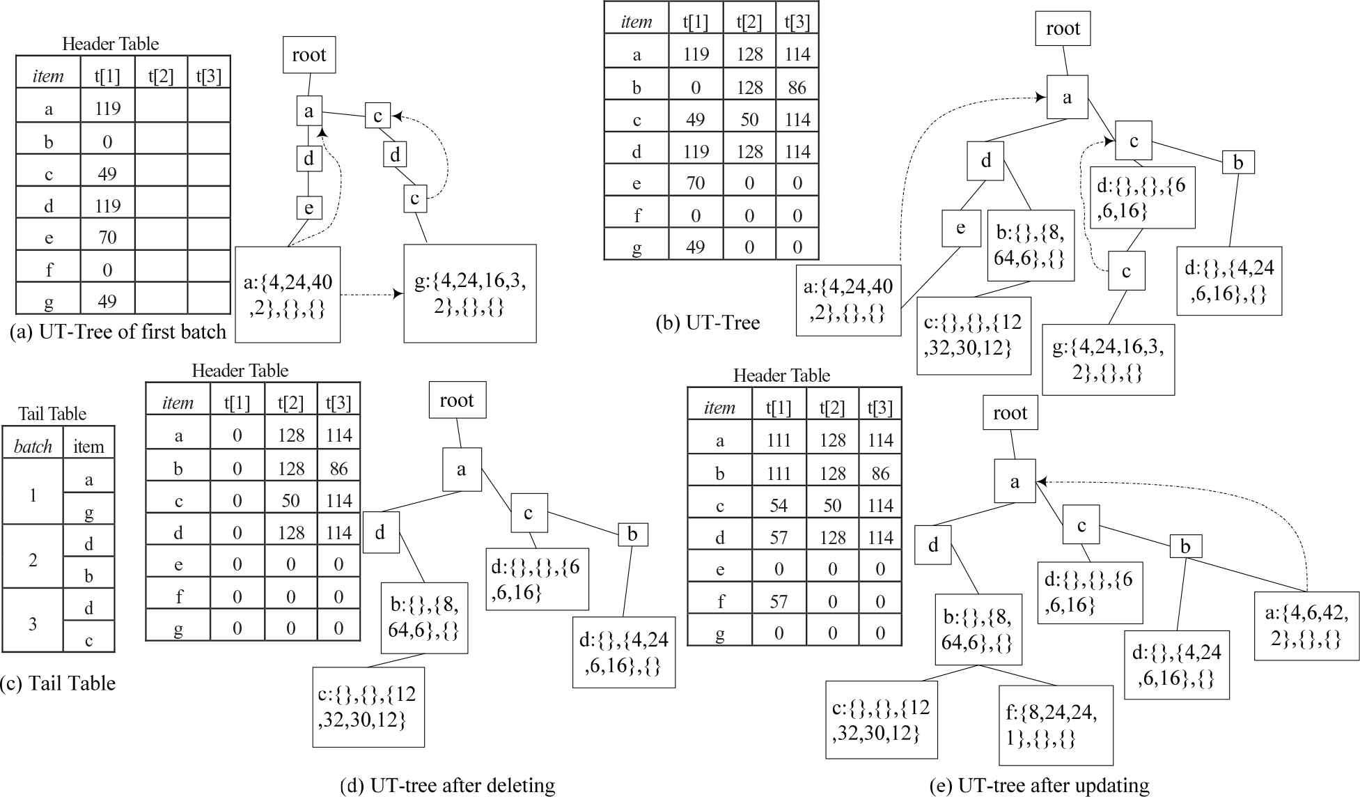
We use an example to illustrate the construction of UT-tree based on the data in Tables 1 and 2. The window size w = 3 and in each batch of data contains two transactions. The first batch of data with transaction t1 and t2 are added to a tree in its original order. Note that the last node of each transaction that is added to the tree is a tail-node, such as the node “a” in the transaction {a, d, e, a} and “g” in the transaction {a, c, d, c, g}, the tail-node records the utility of the items in its transaction. Figure 1(a) is the result of the first batch of two transactions added to a UT-tree. Figure 1(b) shows the final UT-tree after the third batch of data is added. When constructing a UT-tree, if a tail-node which is added to the tree has already being a corresponding ordinary-node, we simply convert this ordinary-node to a tail-node. For example, t5= {a, c, d}, when the transaction is added into the tree, the same path has already existed after adding the transaction t2, but in transaction t5, “d” is the tail-node while it is an ordinary-node in t2, simply convert the node to a tail-node with the utility of t5. The global header table which records the swu of batch in t[1], t[2], and t[3]. The tail table (Figure 1(c)) records the order of the batch which is used to delete obsolete data, we also add the pointer to the node when the item is appeared more than once in the transaction, it is pointed to the same item which is nearest to it. For example, in transaction {a, c, d, c, g}, the second item “c” points to the first “c” for calculating the utility of same item or sequence in the same transactions.
Construction of a UT-Tree.
3.2. Data Updating
When a new batch with two transactions comes, two important processes occur: deleting obsolete data and adding new data.
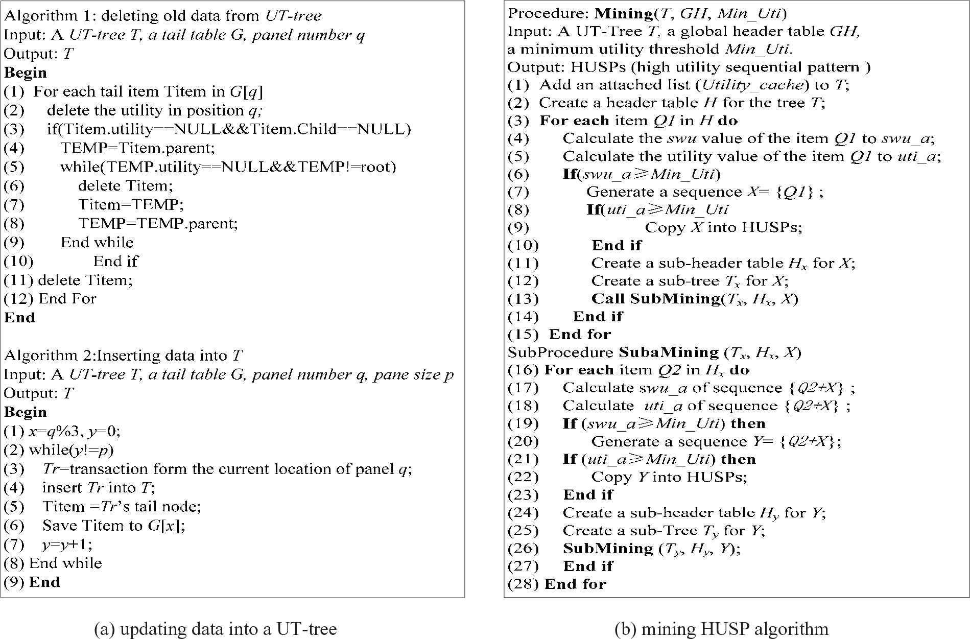
The algorithm of deleting old data is shown in Algorithm 1 of Figure 2(a). Mainly its work is to process each obsolete tail-node which is recorded in the tail table. Delete the utility in the tail-node (line 2), if there is not any utility in the tail-node, delete the whole path (line 3–10), also delete the item in the tail table (line 11). The algorithm for adding new data is shown in algorithm 2 of Figure 2(a). Transactions are added to the tree (line 3–4), then, the nail-node is stored to the tail table (line 6). The variable y in algorithm 2 is the looping counter.
Algorithms based on UT-tree.
For UT-tree in Figure 1(b), when the fourth batch with transaction t7 and t8 comes, Figure 1(d) is the result after deleting the first batch of data and Figure 1(e) is the final result after updating.
3.3. Mining HUSP Algorithm
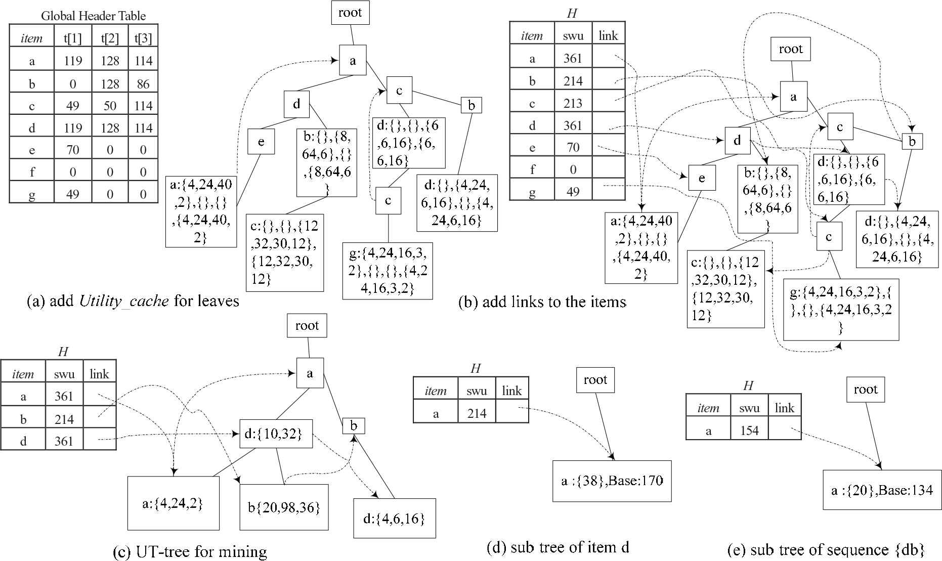
The new mining algorithm is proposed in Figure 2(b). Line 1 in the algorithm is to add a numeric list named Utility_cache to each leaf node on the UT-tree T. The elements in this list are the list of utility for each batch of data on the node (shown as “{}” on the tail-node), for example, for the tree of Figure 1(b), each leaf node adds a list of Utility_cache as shown in Figure 3(a). Line 2 in the algorithm is to create a header table H, and the entries and their order are obtained from global header table GH, scanning the tree and placing all the nodes of the same item in the link of H, the link order of the item is corresponding to the order of the batches. H could be obtained in Figure 3(b) based on the UT-tree and global head table of Figure 3(a).
Process of mining HUSPs from a UT-Tree.
The third to fifteenth lines of the algorithm start from the last item in H and sequentially process each item in H. Lines 4 and 5 calculate swu and utility values of the current processing item based on Utility_cache in the path. From the current processing item, the utility of the same item in another transaction can be obtained based on the links, if the item appears in a path more than once, the utility can be calculated based on definition 1. If the utility value of the current processing item is not less than MinUti, the item is an HUSP (sequence with length 1). If the swu of the item is not less than MinUti, you can create the sub-header table and sub-tree (lines 11 and 12 in the algorithm).
The creation of the sub-header table and sub-tree is described in line 16 and line 25 of Figure 2(b). For example, set MinUti = 214, Figure 3(c) is the final UT-tree after deleting the items whose swu is less than 214, and the tail-nodes of the tree contain the value of Utility_cache. The sub-tree of item “d” could be known from Figure 3(d), the value of base is corresponding to the processing item. To process the item “d” in H of Figure 3(c), there are two paths in the UT-tree. The path “root-a-d” and “root-a-b-d,” the swu values of all items in these two paths are calculated, and the item whose swu is not less than MinUti is stored in a sub-header table, we can find that the sequence {ad} satisfies the demand. Figure 3(e) is the sub-tree corresponding to the sequence {db}.
The 26th line of the algorithm deals with the sub-header table and sub-tree. The process method of sub-header table and sub-tree is the same as the processing method of UT-tree. For details, refer to the lines 1–15 in Figure 2(b).
3.4. Algorithm Analysis
The proposed algorithm HUSP-UT (mining HUSPs-based UT-tree) stores the sequence’s utility in the leaf node. It guarantees HUSP-UT to get the real utility value of the sequence from the UT-tree instead of estimating value, there is no candidates generating in the mining process, the storage consumption is effectively reduced. You can get the utility value of each item in the correlative sequence when creating sub trees (the creation of the sub-tree in Figure 3) based on the node pointer. This is also guaranteed to be able to calculate the utility of items in the head table and the new swu value fast (not contain the utility value of items that have been processed and not in the head table), it reduces the running time efficiently.
It is known that when it is going to create a sub-tree of the item or sequence X, the utility of X is calculated from the global tree and the sequence which contains X could be found based on the sub-tree. The utility can be calculated from a sub-tree to any item or sequence.
The above is the reason for the efficiency improvement of algorithm HUSP-UT, the experimental results are given in Section 4 of this paper.
Below we prove that our method for finding HUSPs does not miss any HUSPs. Firstly assuming the sequence Z is any HUSP mode, than the swu value of any non-empty subset will not be less than the minimum threshold. According to the algorithm HUSP-UT, all items in the sequence Z will appear in the header table corresponding to the UT-tree. When the item Z1 in the sequence Z is processed and the sub-header table is created based on the node pointer, the swu value of Z1 combined with the rest item of Z is not less than the minimum threshold. So these combined item will appear in the sub-tree of Z1. When processing the new item of Z1, it is iteratively calculated according to the same creation rules of the sub-tree, it can definitely get that the sequence Z is the HUSP mode and this algorithm HUSP-UT can mine all HUSPs.
4. EXPERIMENTAL ANALYSES
In this section, we evaluate the performance of the proposed algorithm HUSP-UT (mining HUSPs based UT-tree) and compare it with state-of-the-art HUSP-Stream on four datasets: Bible, FIFA, Kosarak10k, and SIGN. These datasets have varied characteristics and represent the main types of data typically encountered in real-life scenarios (dense, sparse, short, and long sequences). The dataset is obtained from SPNF [21] and paper [22]. The characteristics of datasets are shown in Table 3, where |I|, avgLength, and |SD| columns indicate the number of distinct items, the average sequence length, and number of sequences. Bible is moderately dense and contains many medium-length sequences. FIFA is moderately dense and contains many long sequences. Kosarak10k is a sparse dataset that contains short sequences and a few very long sequences. SIGN is a dense dataset having very long sequences. For all datasets, external utilities of items are generated between 0.01 and 10 by using a lg-normal distribution [23]. All algorithms were written in Java programming language. The configuration of the testing platform is as follows: Windows7 operating system, 2G Memory, intel
| Dataset | |I| | AvgLength | |SD| |
|---|---|---|---|
| Bible | 13 905 | 21.64 | 36 369 |
| FIFA | 13 749 | 45.32 | 573 060 |
| Kosarak10k | 39 998 | 11.64 | 638 811 |
| SIGN | 267 | 93.00 | 730 |
Data characteristics.
(R) Core(TM) i3-2310 CPU@2.10 GHz, Java heap size is 1G. The two methods can mine all HUSPs in the dataset, and we evaluate the time and memory consumption efficiency on the four datasets.
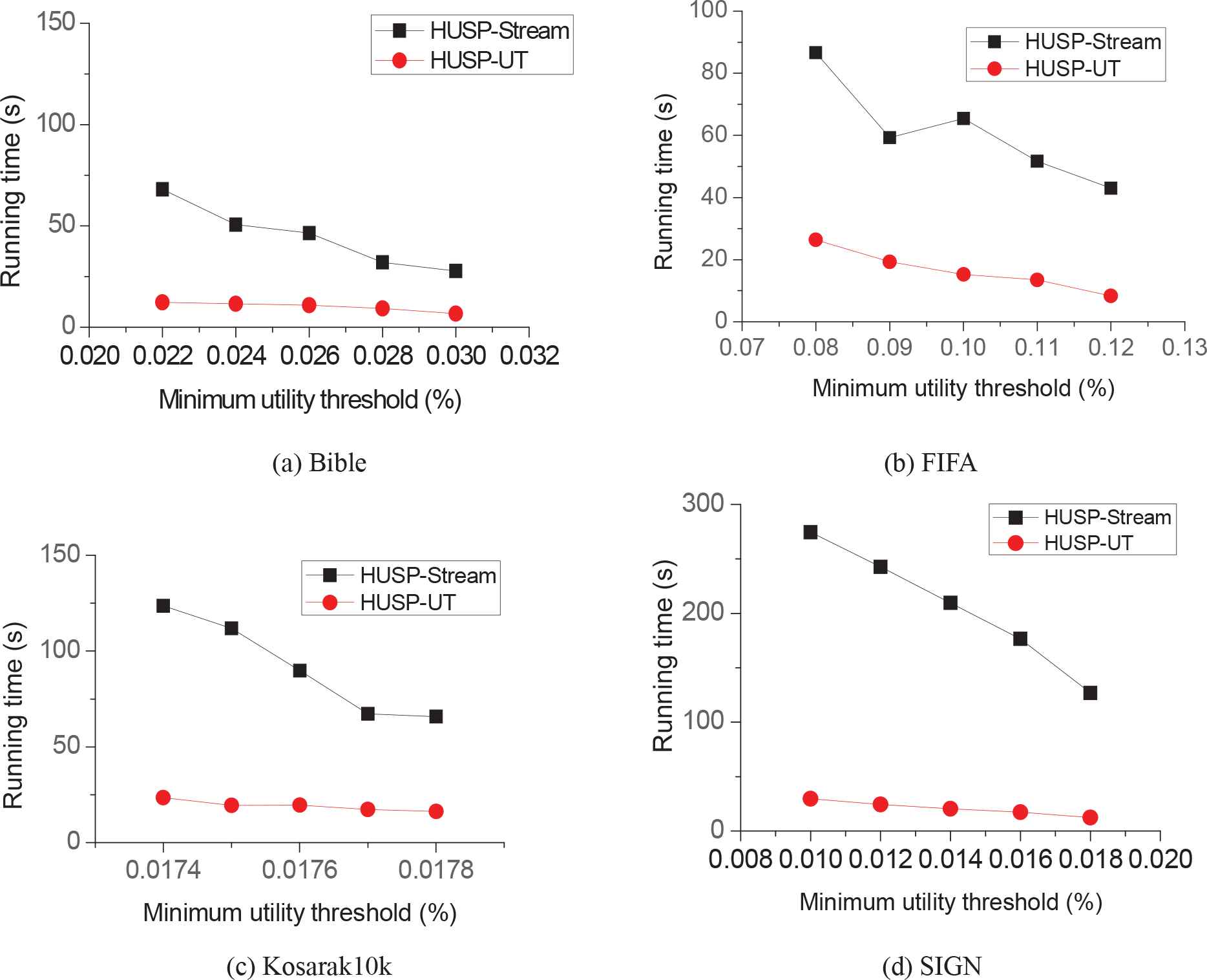
Figure 4 shows the running time comparison of HUSP-UT and HUSP-Stream under four datasets, respectively. The number of data batch is set as w = 3 in each window and the batch-size are set as 10K. From the results on Figure 4, we can see that our algorithm HUSP-UT outperforms HUSP-stream on different minimum support thresholds. For example, when the minimum support threshold is 0.01% on the dataset SIGN, HUSP-UT spends 29.56 seconds while HUSP-stream spends 274.521 seconds. The time efficiency is up to 1 order of magnitude faster on the dataset. There will be more HUSPs when the threshold getting smaller, the total running time will increase along with the decrease of the threshold, but we can see that the running time is stable by HUSP-UT and the efficiency is improved by using the new method.
Execution time under varied minimum utility threshold.
Figure 5 shows the running time comparison for evaluating the accumulated performance of HUSP-UT and HUSP-stream under varied window-width, the minimum utility threshold is set as 0.026%, 0.1%, 0.0174%, and 0.014%, respectively. Each batch-size is 10K, with the increasing of the number of batches in the window, the total running time of HUSP-stream increases more, mainly because it creates more candidates, while the time of HUSP-UT is not very big. The performance advantage of algorithm HUSP-UT accumulates along with window-width, it is stable under varied window-width.
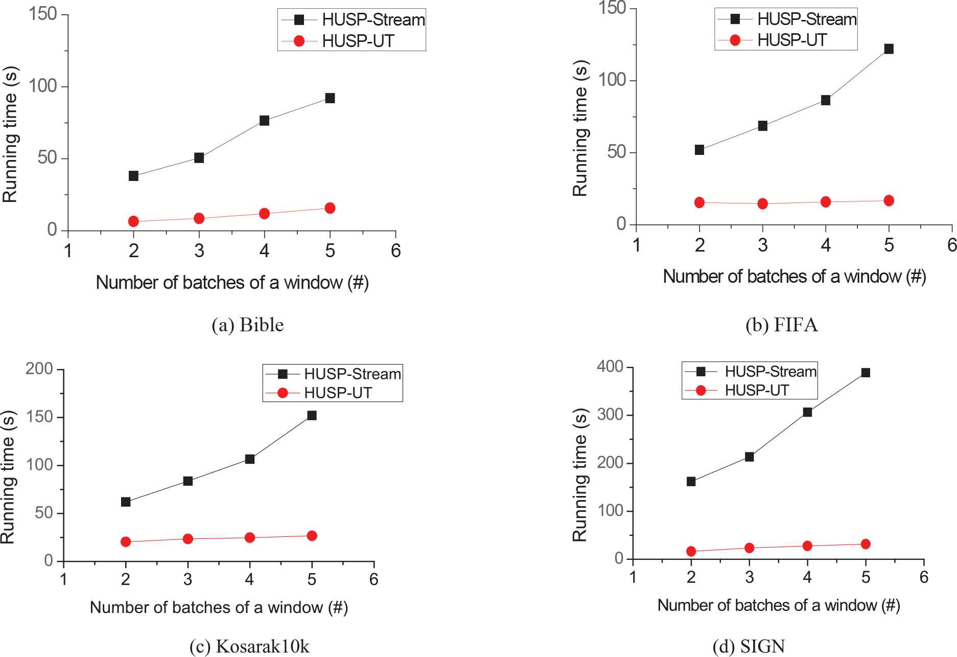
Execution time under varied window-width.
Figure 6 shows that our algorithm HUSP-UT outperforms HUSP-stream on varied batch-sizes. In Figure 6, the minimum utility threshold was set to 0.026%, 0.1%, 0.0174%, and 0.014%, respectively. The window size was three batches, and the batch-size test range was 5K–25K. The results of this experiment are the same as the above experiments. The time performance of HUSP-UT is still better than that of HUSP-stream.
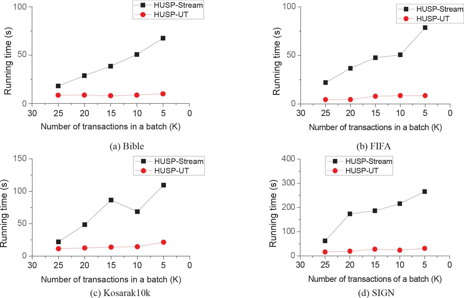
Execution time under varied batch-size.
We also evaluate the memory usage of the algorithms under different utility thresholds. The number of data batch is set 3 in each window and the batch-size is set as 10K, the results are shown in Figure 7, which indicates our approach consumes less memory than HUSP-stream. For example, for the dataset FIFA, when the threshold is 0.026%, the memory consumption of HUSP-UT is around 200 MB, while that of HUSP-Stream is over 500 MB. A reason is that HUSP-Stream produces too many candidates during the mining process, which causes HUSP-Stream having a larger tree than that of HUSP-UT.
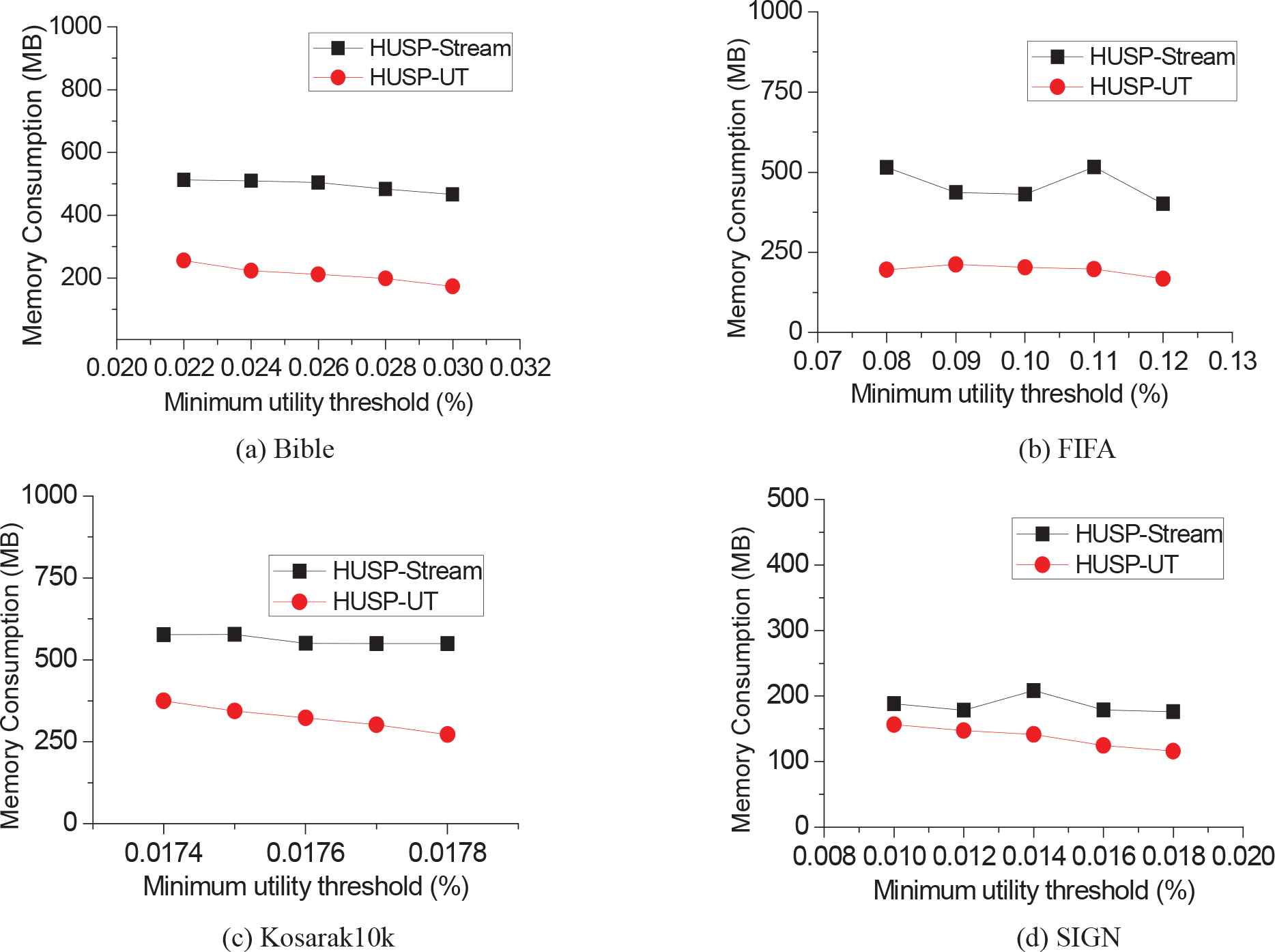
Memory consumption on four datasets.
The performance of the algorithms under different window sizes and batch number are also evaluated in this experiment, the minimum utility threshold is set to 0.026%, 0.1%, 0.0176%, and 0.014% for the four datasets, respectively. The results are shown in Figure 8. In Figure 8(a), each bar shows the memory consumption of HUSP-UT on a dataset under a window size when the number of batches is three. For example, the most left bar is the memory consumption of HUSP-UT on Bible when the window size is set to 10K. From Figure 8(a), we observe that the memory consumption of HUSP-UT increases very slowly with increasing window sizes.
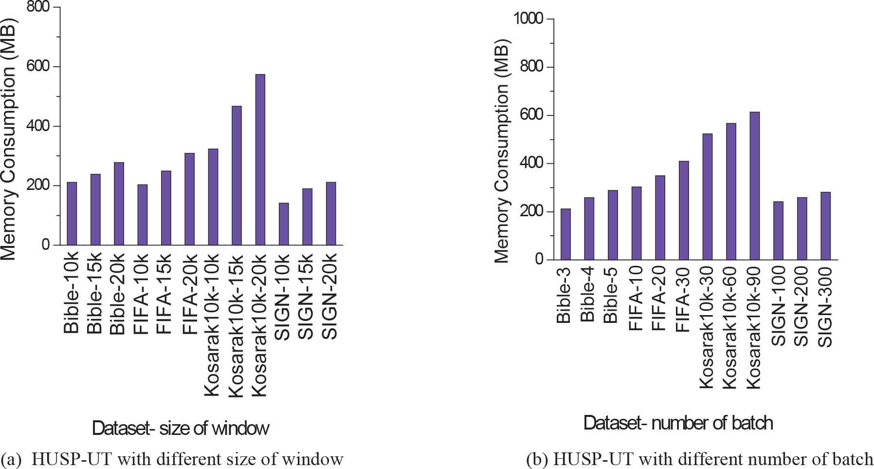
Evaluation of high utility sequential pattern utility on Tail Tree (HUSP-UT).
Figure 8(b) shows the memory consumption of HUSP-UT under different batch number when the size of a window is 10K, the dataset with different number is displayed with the abscissa. For example,“Bible-3” indicates that there are three batches of transactions in a window with the dataset Bible. We also see that the memory consumption of HUSP-UT increases very slowly with increasing number of batches in a window.
Concluding the above experiments, we can see that our proposed algorithm HUSP-UT has achieved a better performance than HUSP-stream under varied minimum support thresholds, varied window-width, and varied batch-sizes, and its advantage is stable along with the accumulation of the data flow process.
5. CONCLUSIONS
To improve the overall performance of the high utility sequence mining algorithm over DSs, the efficiency of updating data and mining HUSP should be considered. This study proposes a new data structure UT-tree and gives the corresponding algorithm HUSP-UT. We apply the new method to mine HUSPs over DSs. Theoretical and experimental analysis shows that the performance of our proposed algorithm outperforms the state-of-the-art algorithm HUSP-Stream.
ACKNOWLEDGMENTS
This work is supported by the Project of Zhejiang Provincial Public Welfare Technology Application and Research (LGF19H180002, 2017C35014) and Ningbo Natural Science Foundation (2017A610122).
REFERENCES
Cite this article
TY  - JOUR
AU  - Huijun Tang
AU  - Yangguang Liu
AU  - Le Wang
PY  - 2019
DA  - 2019/01/28
TI  - A New Algorithm of Mining High Utility Sequential Pattern in Streaming Data
JO  - International Journal of Computational Intelligence Systems
SP  - 342
EP  - 350
VL  - 12
IS  - 1
SN  - 1875-6883
UR  - https://doi.org/10.2991/ijcis.2019.125905650
DO  - 10.2991/ijcis.2019.125905650
ID  - Tang2019
ER  -
