
Local Linear Regression Estimator on the Boundary Correction in Nonparametric Regression Estimation
- DOI
- 10.2991/jsta.d.201016.001How to use a DOI?
- Keywords
- Kernel estimators; Nonparametric regression estimation; Local linear regression; Bias; Variance; Asymptotic mean integrated square error (AMISE)
- Abstract
The precision and accuracy of any estimation can inform one whether to use or not to use the estimated values. It is the crux of the matter to many if not all statisticians. For this to be realized biases of the estimates are normally checked and eliminated or at least minimized. Even with this in mind getting a model that fits the data well can be a challenge. There are many situations where parametric estimation is disadvantageous because of the possible misspecification of the model. Under such circumstance, many researchers normally allow the data to suggest a model for itself in the technique that has become so popular in recent years called the nonparametric regression estimation. In this technique the use of kernel estimators is common. This paper explores the famous Nadaraya–Watson estimator and local linear regression estimator on the boundary bias. A global measure of error criterion-asymptotic mean integrated square error (AMISE) has been computed from simulated data at the empirical stage to assess the performance of the two estimators in regression estimation. This study shows that local linear regression estimator has a sterling performance over the standard Nadaraya–Watson estimator.
- Copyright
- © 2020 The Authors. Published by Atlantis Press B.V.
- Open Access
- This is an open access article distributed under the CC BY-NC 4.0 license (http://creativecommons.org/licenses/by-nc/4.0/).
1. INTRODUCTION
In nonparametric estimation, one aspect that is of importance is the smoothing that makes the interpretation of data possible. Smoothing in essence, consists of creating an approximating function that attempts to capture only the important patterns, while filtering noise and ignoring the data structures that are deemed not relevant [1]. This nonparametric technique is applicable both to density and regression estimation. Other common techniques in nonparametric regression estimation, the focus in this paper, are the spline regression, orthogonal series, and kernel regression. This paper explores the kernel regression estimation under the larger framework of the model-based estimation. One motivating research is due to Dorfman [2] who used the Nadaraya–Watson estimator also known as the local constant to construct the finite population estimator. Even with this boundary drawback, the estimator of the population total was still better than the Design-based Horvitz–Thompson estimator [3]. Many researchers in the past have done studies incorporating the Nadaraya–Watson technique. A few examples include Hall and Presnel [4], Cai [5], and Salha and Ahmed [6] who carried out a study about this. They proposed a weighted Nadaraya–Watson estimator for use in the context of conditional distribution estimation. In their studies they found out that weighted Nadarya–Watson was an improvement. In particular Cai [5] claimed that it was easier to implement Nadaraya–Watson estimator than the local linear. Herbert et al. [7] in their study suggested using jackknife technique to improve the Nadaraya–Watson estimator for finite population total. Generally, it is however known in literature, that the standard Nadaraya–Watson estimator suffers from the boundary bias and as a result the prime focus in this study is the boundary correction using the local linear estimator.
This paper has been organized as follows: in Section 2, we give a brief review of the literature regarding nonparametric regression and kernel regression estimation. In Section 3, we derive the bias and the variance of Nadaya–Watson and local linear regression estimators. The boundary correction shall be shown in this section as well. Empirical analysis has been done in Section 4 using some artificially simulated datasets. Discussion of results and conclusion is given in Section 5.
2. LITERATURE REVIEW
In this section review of literature on nonparametric regression estimation has been done. Also included in this section is the literature on kernel regression estimators.
2.1. Nonparametric Regression Estimation
Nonparametric regression estimation has been carried out by many researchers in many studies. Dorfman [2] did a comparison between the famous design-based Horvitz–Thompson estimator and the nonparametric regression estimator developed by using Nadaraya–Watson estimator [8,9]. In his study, he found out that the kernel-based nonparametric regression estimator better reflects the structure of the data and hence yields greater efficiency. This regression estimator, however, suffered the so-called boundary bias besides facing bandwidth selection challenges. Breidt and Opsomer [10] did a similar study on nonparametric regression estimation of finite population under two-stage sampling. Their study also reveals that the nonparametric regression with the application of local polynomial regression technique dominated the Horvitz–Thompson estimator and improved greatly the Nadaraya–Watson estimator. Breidt et al. [11] in their results also show that the nonparametric regression estimation is superior to the standard parametric estimators when the model regression function is incorrectly specified, while being nearly as efficient when the parametric specification is correct.
2.2. AMISE in Kernel Regression Estimators
The key properties that a statistician would be interested to check given an estimator are the variance and the bias. These two can enable one to measure the amount of accuracy and precision that an estimator has. In fact at an arbitrary fixed point, a basic measure of accuracy that takes into account both the bias and variance is the mean square error (MSE), Tsybakov [12], Härdle [13], Takezawa [14], and Härdle et al. [15]. In nonparametric regression estimation, one would be interested in the cumulative amount of bias and the variance over the entire regression line. This global measure called mean integrated square error (MISE) is obtained by finding the integral value of the variance and the square of the bias of the estimator over the entire line [16]. Taylors' expansion is normally used to obtain the asymptotic mean integrated square error (AMISE). Using differential calculus an optimal bandwidth can be obtained based on this AMISE. Among researchers who have carried out studies using these measures include Manzoor et al. [17]. Given the asymptotic properties one can deduce the speed of convergence of the estimators and determine the price to pay in a given option. It is from this literature that in Section 3, this study uses these measures in the analysis stage to compare the proposed estimator against the standard ones reported.
3. METHODOLOGY
This section gives the various techniques that have been used in this study to perform the regression estimation. More specifically the properties of each of the estimators have been given.
3.1. Properties of the Kernel Regression Estimators
A model-based nonparametric model is conventionally of the form
Yi is the variable of interest
Xi is the auxiliary variable
m is an unknown function to be determined using sample data
ei is error term-assumed to be
The pairs of (Xi, Yi) is a 2-dimensional bivariate random variables in the sample space.
The idea of nonparametric regression has gained prominence in a couple of decades now. The recent advancement in technology and computers has enabled researchers to handle the massive computation experienced with this approach. This section gives a brief derivation of Nadaraya–Watson estimator.
3.2. Review of the Nadaraya–Watson Estimator
Let K(.) denote a kernel function which is also twice continuously differentiable, such that
Further, let the smoothing weight with a bandwidth h be
Assume a model of the form specified in (1), the Nadaraya–Watson estimator of m(x) is therefore given by
Incorporating the Gaussian kernel function the value of
This gives a way of estimating the nonsample values of y given x the auxiliary value. The nonparametric estimator for the finite population total is thus given by
The equation in (6) was first suggested by Dorfman [2]. For kernel regression estimator, the estimate of m at point x is obtained using a weighted function of observations in the h-neighborhood of x. The weight given to each observation in the neighborhood depends on the choice of kernel function.
For example a uniform kernel function would assign the same weights to all the points within its window while the bi-weight kernel function on the other hand, assigns more weight to the points closest to the target and diminishes the weights in those points that are “farthest away” from the center of the kernel.
Choosing an appropriate kernel and a suitable bandwidth is quite important in nonparametric regression. It is known that the two (i.e., kernel function and the bandwidth), do not have the same effects—in terms of their contribution in the estimate. Previous studies reveal that compared to the kernel function which has the least impact while bandwidth selection plays a more crucial part in obtaining good estimates [18].
3.2.1. Properties of the Nadaraya–Watson estimator
The bias term of a Nadaraya–Watson estimator can be shown to be given by
The variance term can be shown to be
The proofs of these terms have not been done in this paper. Readers who may be interested can refer to [19]. A critical look at these properties shows that the bandwidth h is directly proportional to the bias while being inversely proportional to the variance. This implies that larger a value of h increases the size of the bias but at the same time reduces the variance. The opposite is true for small value of the bandwidth. See Figure 1 for an insight of this. From this fact, it is obvious that an optimal bandwidth that minimizes the AMISE measurement criterion is required.
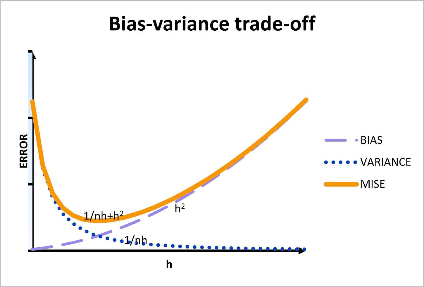
Impact of the bandwidth on variance and the bias.
3.2.2. Optimal bandwidth of the Nadaraya–Watson estimator
The bandwidth that optimizes Nadaraya–Watson estimator can be found by minimizing the AMISE function given in (10) with respect to h. The first derivative is given by
Equating this to zero and solving for h yields an optimal bandwidth,
3.3. Review of the Local Polynomial Regression Estimator
Let (X1, Y1), (X2, Y2), …, (Xn, Yn) be a random sample of a bivariate data taken from a finite population. From the model in (1), to estimate the unknown function m(Xi), the procedure below follows:
This can be approximated using Taylor's series as
This gives the weighted LSE having the weights:
So that letting
i.e.,
The degree of the local polynomial regression has an implication on the estimate in terms of how it addresses the boundary and the interior biases as well as the effect on variance. The polynomials of degree more than three have been known to reduce the bias much more the local linear at the interior but at the cost of high variance. The same local polynomials however, are poorer at the boundary. It is also known that the odd order degree dominate those of even order. From there researches it can be concluded that it suffices to keep the order of the local polynomial regression low and concentrate on adjusting the bandwidth. Härdle et al. [15] and Avery [21] among others can be referred for this. Because of this fact, this study confines itself to the local linear regression estimation which is achieved from the local polynomial regression of degree one. It is of interest to note that Nadaraya–Watson estimator is a special case of the local polynomial regression estimator with the degree kept at zero.
3.3.1. The properties of local linear regression estimator
In this paper the properties of this estimator have been stated. More detailed theoretical derivations can be found in [15].
The bias of local linear regression is given by
While the conditional variance is given by
Thus the MSE of
Integrating the MSE in (17) gives us the MISE of the local linear estimator. This is given by
Hence the asymptotic MISE is
3.3.2. The optimal bandwidth for the local linear regression estimator
As it was done with the local constant the optimal bandwidth for the local linear estimator can be obtained by minimizing the expression in (19) to have
Solving this for the bandwidth, h;
The application of these optimal bandwidths can generally be challenging because there are a number of unknown functions that require estimation first such as the marginal density
4. EMPIRICAL STUDY
Data simulation was done using the model in (1) so that
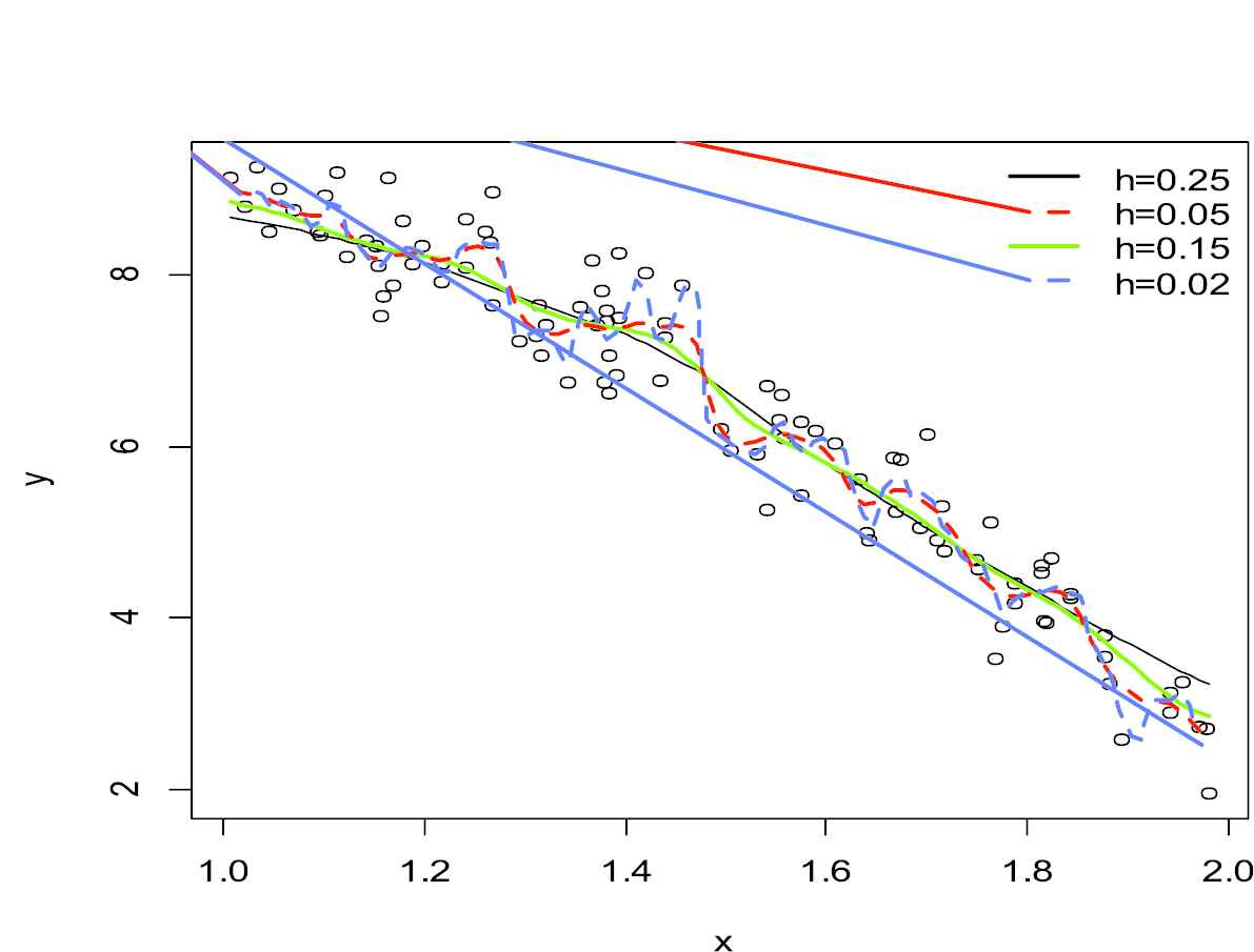
Nadaraya–Watson estimator with varying bandwidths.
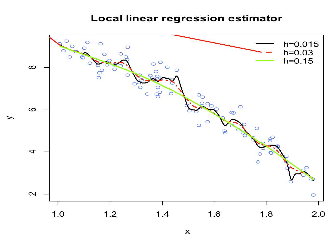
Local linear estimator with varying bandwidths.
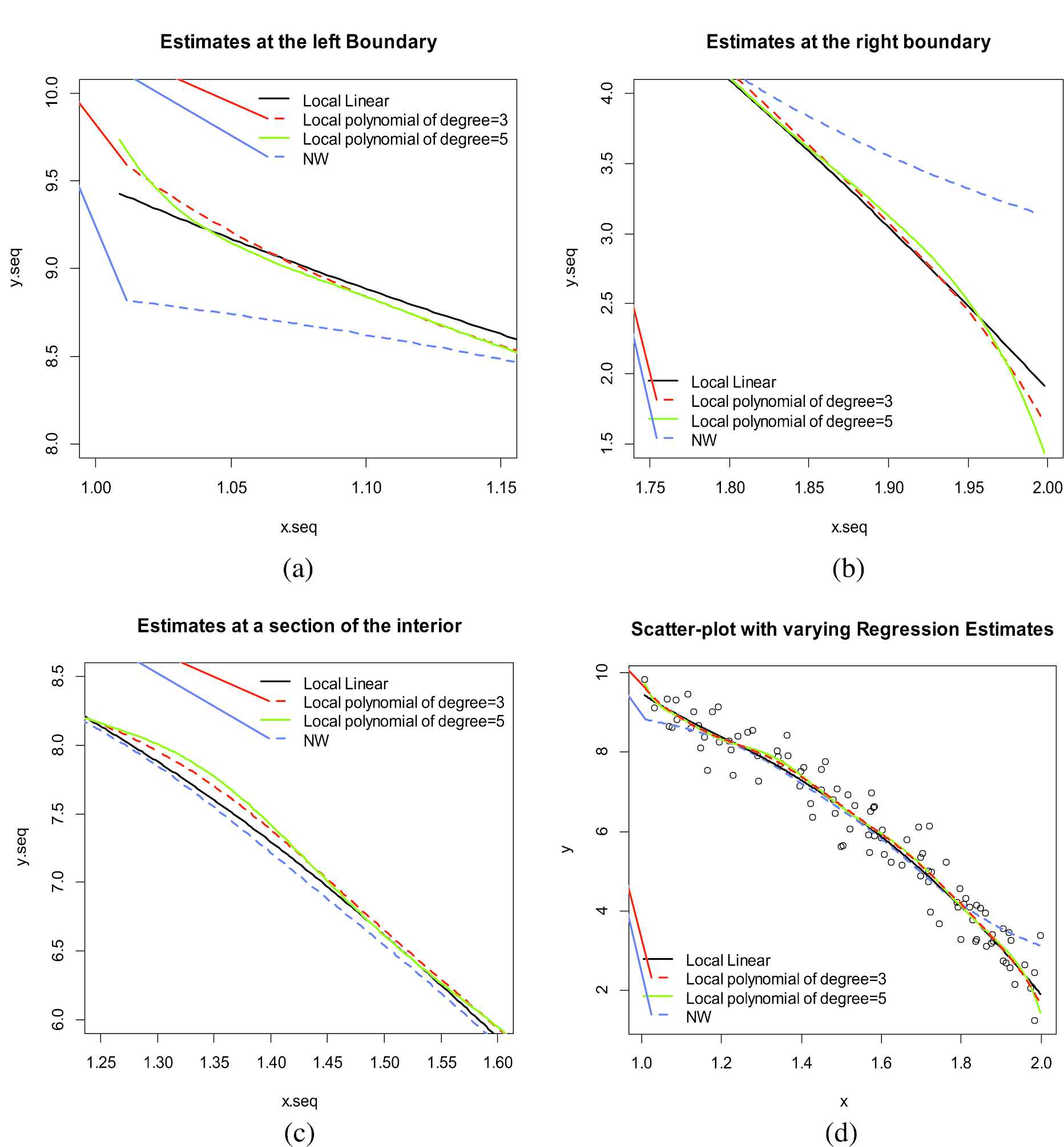
Boundary and interior bias-variance trade-off in regression estimates. Graphs (a)-(c) are specific portions of the graph given in part (d).
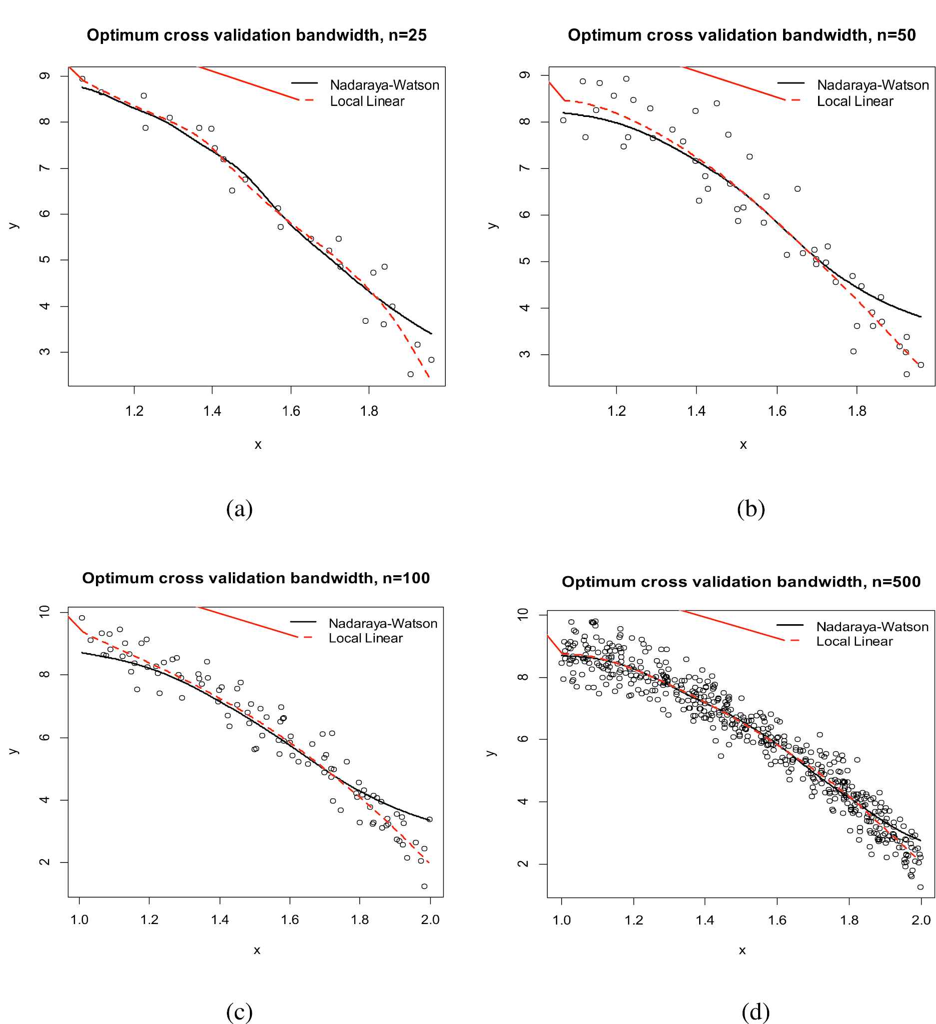
Comparing the standard Nadaraya–Watson estimator and the local linear regression techniques with varying sample sizes and optimal bandwidths.
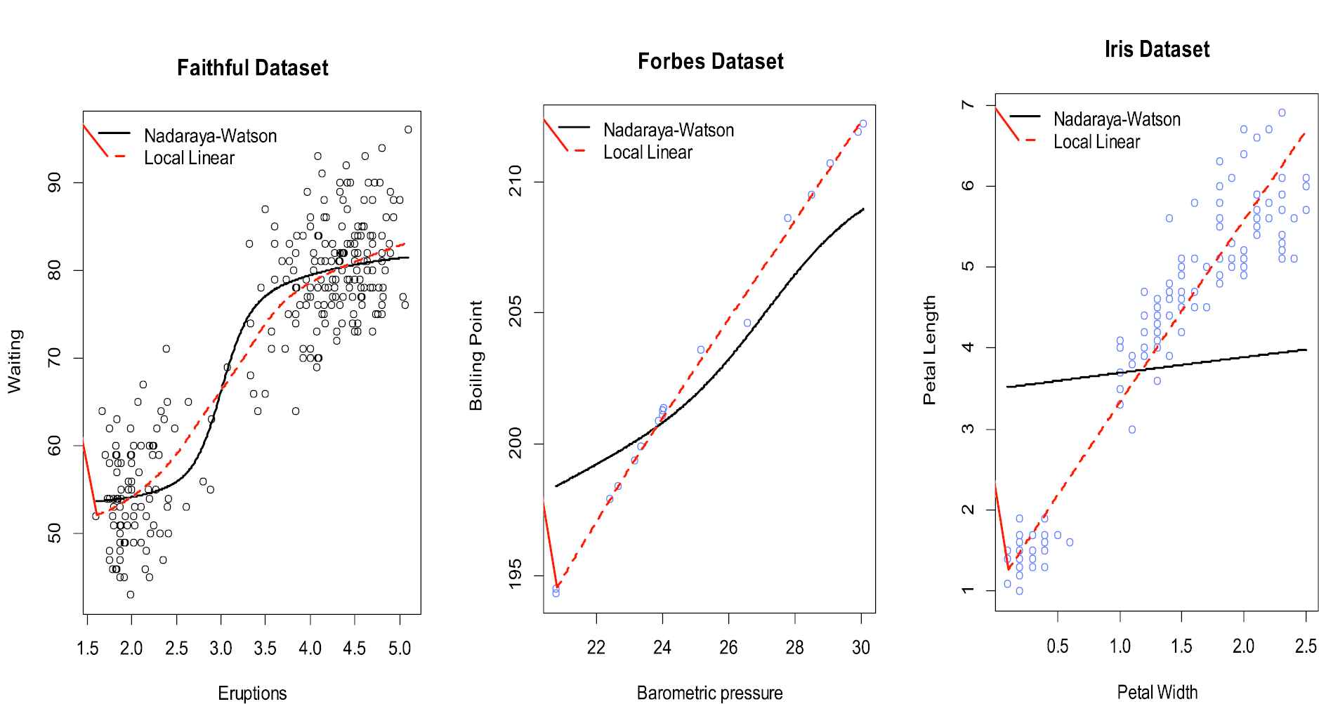
Comparing the standard Nadaraya–Watson estimator and the local linear regression techniques using inbuilt datasets in R.
| Model | Equation |
|---|---|
| 1: Cubic | |
| 2: Bump | |
| 3: Quadratic | |
| 4: Linear | |
| 5: Exponential |
Models used in simulation.
| Dataset | Nature of Boundary Bias | Estimator | AMISE | h AMISE |
|---|---|---|---|---|
| Faithful dataset | No boundary correction | NW | 0.00027040 | 7.781472 |
| Boundary corrected | LL | 0.00024807 | 7.375393 | |
| Forbes dataset | No boundary correction | NW | 0.00075248 | 2.278702 |
| Boundary corrected | LL | 0.00043041 | 3.537160 | |
| Iris dataset | No boundary correction | NW | 0.01650655 | 0.093106 |
| Boundary corrected | LL | 0.00141712 | 1.083385 |
Asymptotic mean integrated square error (AMISE) for the standard Nadaraya–Watson (NW) kernel estimator and local linear (LL) regression estimator computed for various selected datasets.
5. CONCLUSION AND RECOMMENDATION
From the results of the simulated data presented in the respective figures, it is clear that the local linear estimator does not induce the boundary bias into its estimate as is the case with the Nadaraya–Watson estimator. In addition it was revealed from Figure 4 that while the increment of the degree of the local polynomial seems to be reducing the interior bias, the unfortunate result is that it came with a cost of higher variance. They also do not perform adequately at the boundary as the local linear does. The superior performance of the local linear estimator also manifested itself in the figures obtained using various inbuilt datasets in r (see Table 2). Local linear estimator can therefore be recommended for removal of the boundary bias. If however the problem is the interior bias then with proper adjustment of the bandwidth may suffice in some cases. The gains made by moving to higher order degree are insignificant. It is also clear that for both cases the bandwidth play a significant role as a smoothing parameter and thus proper selection should be born in mind during estimation. These facts were supported by the overall smaller values of AMISEs for the local linear estimator that proved to be superior in all aspects to the Nadaraya–Watson estimator as seen from the results given in Tables 2–7.
| Sample Size | Nature of Boundary Bias | Estimator | AMISE | h AMISE |
|---|---|---|---|---|
| n = 25 | No boundary correction | NW | 0.001677 | 1.169522 |
| Boundary corrected | LL | 0.001348 | 1.201303 | |
| n = 50 | No boundary correction | NW | 0.001721 | 1.063632 |
| Boundary corrected | LL | 0.001402 | 1.206711 | |
| n = 100 | No boundary correction | NW | 0.001401 | 1.211507 |
| Boundary corrected | LL | 0.001119 | 1.453101 | |
| n = 500 | No boundary correction | NW | 0.001291 | 1.316334 |
| Boundary corrected | LL | 0.001218 | 1.375686 | |
| n = 1000 | No boundary correction | NW | 0.001254 | 1.353020 |
| Boundary corrected | LL | 0.001200 | 1.398421 |
Asymptotic mean integrated square error (AMISE) for the standard Nadaraya–Watson (NW) kernel estimator and local linear (LL) regression estimator (Model 1-Cubic function).
| Sample Size | Nature of Boundary Bias | Estimator | AMISE | h AMISE |
|---|---|---|---|---|
| n = 25 | No boundary correction | NW | 0.005367 | 0.288393 |
| Boundary corrected | LL | 0.004966 | 0.309645 | |
| n = 50 | No boundary correction | NW | 0.005475 | 0.305584 |
| Boundary corrected | LL | 0.004082 | 0.375665 | |
| n = 100 | No boundary correction | NW | 0.005138 | 0.309597 |
| Boundary corrected | LL | 0.003956 | 0.384638 | |
| n = 500 | No boundary correction | NW | 0.004921 | 0.340515 |
| Boundary corrected | LL | 0.003893 | 0.394235 | |
| n = 1000 | No boundary correction | NW | 0.004774 | 0.347761 |
| Boundary corrected | LL | 0.003845 | 0.399115 |
Asymptotic mean integrated square error (AMISE) for the standard Nadaraya–Watson (NW) kernel estimator and local linear (LL) regression estimator (Model 2-Bump function).
| Sample Size | Nature of Boundary Bias | Estimator | AMISE | h AMISE |
|---|---|---|---|---|
| n = 25 | No boundary correction | NW | 0.002797 | 0.576798 |
| Boundary corrected | LL | 0.002641 | 0.609480 | |
| n = 50 | No boundary correction | NW | 0.002446 | 0.685321 |
| Boundary corrected | LL | 0.002169 | 0.740991 | |
| n = 100 | No boundary correction | NW | 0.002288 | 0.716167 |
| Boundary corrected | LL | 0.002135 | 0.759066 | |
| n = 500 | No boundary correction | NW | 0.002085 | 0.787549 |
| Boundary corrected | LL | 0.002040 | 0.799239 | |
| n = 1000 | No boundary correction | NW | 0.002057 | 0.797407 |
| Boundary corrected | LL | 0.002029 | 0.804035 |
Asymptotic mean integrated square error (AMISE) for the standard Nadaraya–Watson (NW) kernel estimator and local linear (LL) regression estimator (Model 3-Quadratic function).
| Sample Size | Nature of Boundary Bias | Estimator | AMISE | h AMISE |
|---|---|---|---|---|
| n = 25 | No boundary correction | NW | 0.005368 | 0.2883934 |
| Boundary corrected | LL | 0.004966 | 0.3096449 | |
| n = 50 | No boundary correction | NW | 0.004253 | 0.3672427 |
| Boundary corrected | LL | 0.004097 | 0.3749881 | |
| n = 100 | No boundary correction | NW | 0.004018 | 0.3782936 |
| Boundary corrected | LL | 0.003928 | 0.3845499 | |
| n = 500 | No boundary correction | NW | 0.003970 | 0.3903203 |
| Boundary corrected | LL | 0.003889 | 0.3943235 | |
| n = 1000 | No boundary correction | NW | 0.003943 | 0.3958703 |
| Boundary corrected | LL | 0.003845 | 0.3990102 |
Asymptotic mean integrated square error (AMISE) for the standard Nadaraya–Watson (NW) kernel estimator and local linear (LL) regression estimator (Model 4-Linear function).
| Sample Size | Nature of Boundary Bias | Estimator | AMISE | h AMISE |
|---|---|---|---|---|
| n = 25 | No boundary correction | NW | 0.647323 | 0.0029467 |
| Boundary corrected | LL | 0.613482 | 0.0031301 | |
| n = 50 | No boundary correction | NW | 0.723391 | 0.0025802 |
| Boundary corrected | LL | 0.635071 | 0.0030013 | |
| n = 100 | No boundary correction | NW | 0.749663 | 0.0027027 |
| Boundary corrected | LL | 0.697904 | 0.0029576 | |
| n = 500 | No boundary correction | NW | 0.673946 | 0.0030442 |
| Boundary corrected | LL | 0.646734 | 0.0031898 | |
| n = 1000 | No boundary correction | NW | 0.699661 | 0.0030770 |
| Boundary corrected | LL | 0.648226 | 0.0031890 |
Asymptotic mean integrated square error (AMISE) for the standard Nadaraya–Watson (NW) kernel estimator and local linear (LL) regression estimator (Model 5-Exponential function).
CONFLICT OF INTEREST
None
AUTHORS' CONTRIBUTIONS
The study has elaborated clearly on the source of the bias in Nadaraya-Watson estimator and how the Local Linear estimator addresses the problem.
Funding Statement
I have solely funded the research by myself. This is an article that i did it alone.
ACKNOWLEDGMENTS
I wish to acknowledge my parent and family members for the support and encouragement. I also appreciate my colleagues at the Department for challenging me to carry out this research.
REFERENCES
Cite this article
TY  - JOUR
AU  - Langat Reuben Cheruiyot
PY  - 2020
DA  - 2020/10/23
TI  - Local Linear Regression Estimator on the Boundary Correction in Nonparametric Regression Estimation
JO  - Journal of Statistical Theory and Applications
SP  - 460
EP  - 471
VL  - 19
IS  - 3
SN  - 2214-1766
UR  - https://doi.org/10.2991/jsta.d.201016.001
DO  - 10.2991/jsta.d.201016.001
ID  - Cheruiyot2020
ER  -