In this paper, we introduce a fractional Generalized Hyperbolic process, a new stochastic process with long-range dependence obtained by subordinating fractional Brownian motion to a fractional Generalized Inverse Gaussian process. The basic properties and covariance structure between the elements of the processes are discussed, and we present numerical methods to generate the sample paths for the processes.
The fractional Brownian motion {BH(t)}t≥0 with Hurst parameter H∈(0,1) is a continuous zero mean Gaussian process with stationary increments and covariance function
CovBH(t),BH(s)=12|t|2H+|s|2H−|t−s|2H,fort,s∈ℝ.
For H=1∕2, the fractional Brownian motion is the same as ordinary Brownian motion which has independent increments. The fractional Brownian motion is first introduced by Mandelbrot and Van Ness [1] and has been widely used in many areas, such as theoretical physics, probability, hydrology, biology, finance, and many others, due to growing interest in the simulation of long-range dependence processes. In finance, especially, as a subclass of the fractional Stable process (See Samorodnitsky and Taqqu [2]), it has been applied to financial time series models having long-range dependence (See Willinger et al. [3], Lo [4], Cutland et al. [5]). Indeed, Kim [6] introduces the fractional multivariate Normal Tempered Stable process by using the time-changed fractional Brownian motion with the fractional Tempered Stable subordinator. Kim [7] redefines a fractional multivariate Normal Tempered Stable process and constructs new market model by applying the process to innovations on the multivariate ARMA-GARCH model.1 Furthermore, Kim et al. [10] use a fractional Tempered Stable process in option pricing and compare its performance with that of the models using other types of stochastic processes. Other than Tempered Stable process, Meerschaert et al. [11] obtains fractional Laplace motion by subordinating fractional Brownian motion to a Gamma process to model hydraulic conductivity fields in geophysics, and Kozubowski et al. [12] applies it to modeling financial time series. Fractional Normal Inverse Gaussian process is also proposed as a simple alternative to the Normal Inverse Gaussian process with long-range dependence (See Kumar et al. [13], Kumar and Vellaisamy [14]).
Financial data have typically exhibited distinct nonperiodic cyclical patterns which are indicative of the presence of long-range dependence. In this paper, we introduce a fractional Generalized Hyperbolic process, a new stochastic process with the long-range dependence. The process is defined by taking the fractional Brownian motion that replaces the time variable to a fractional Generalized Inverse Gaussian process. It is noted that using the time-changed fractional Brownian motion with another long-range dependent stochastic process makes it possible to capture endogenous as well as exogenous long-range dependence (See Kim [6]). We discuss the basic properties of this process and obtain covariance structure between two elements of the processes from the covariance matrix of the fractional multivariate Brownian motion.
Our paper is organized as follows: In Section 2, we review Generalized Inverse Gaussian distribution. In Section 3, the fractional Generalized Inverse Gaussian process is defined, and its basic properties are discussed. In Section 4, we study the corresponding fractional univariate Generalized Hyperbolic process and discuss long-range dependence. Section 5 is devoted to the presentation of the fractional multivariate Generalized Hyperbolic process. In Section 6, we simulate the fractional Generalized Hyperbolic processes and illustrate sample paths for representative values of parameters. The principal findings are summarized in Section 7.
2. GENERALIZED INVERSE GAUSSIAN DISTRIBUTION
The class of Generalized Inverse Gaussian distribution which has been extensively studied by Jørgensen [15] is described by three parameters (λ,δ,γ). Its density function has support on the positive axis and is given by
fGIG(x)=(γ∕δ)λ2Nλ(δγ)xλ−1exp−12δ2x−1+γ2x,x>0,(1)
where Nλ is the modified Bessel function of the second kind with index λ given by Nλ(x)=∫0∞uλ−1e−12x(u−1+u)du for x>0. The parameter domain of the Generalized Inverse Gaussian distribution is
δ>0,γ≥0,ifλ<0,δ>0,γ>0,ifλ=0,δ≥0,γ>0,ifλ>0.
If λ=−12, the density function in Equation (1) reduces to that of the Inverse Gaussian distribution. The Gamma distribution is a limiting case of the Generalized Inverse Gaussian distribution for λ>0 and γ>0 and δ→0. The mean and the variance of a Generalized Inverse Gaussian random variable G can easily be obtained from the Laplace transform. They are given, respectively, by E[G]=δγNλ+1(δγ)Nλ(δγ) and Var(G)=δ2γ2Nλ+2(δγ)Nλ(δγ)−Nλ+12(δγ)Nλ2(δγ). Proposition 2.1 defines characteristic function of the Generalized Inverse Gaussian G.
Proposition 2.1.
The characteristic function of a Generalized Inverse Gaussian random variableGis given by
ϕG(u)=γγ2−2iuλNλ(δγ2−2iu)Nλ(δγ),δ,γ>0.
Proof.
Let q(λ,δ,γ)=γδλ12Nλ(δγ) denote the norming constant of the Generalized Inverse Gaussian density, then the characteristic function of G is
Since Generalized Inverse Gaussian distribution is infinitely divisible, we can define one Lévy process {G(t)}t≥0 such that the characteristic function of G(t) is given by ϕG(t)(u)=E[exp(iuG(t))]=exp(tlog(ϕG(u))), where ϕG(u) is given by Proposition 2.1. In this case, {G(t)}t≥0 is referred to as Generalized Inverse Gaussian process with parameters (λ,δ,γ).
3. FRACTIONAL GENERALIZED INVERSE GAUSSIAN PROCESS
To define a fractional Generalized Inverse Gaussian process, we use the Voltera kernel KH:[0,∞]×[0,∞]→[0,∞], given by
According to Houdre and Kawai [16] and Nualart [17], we have the following facts:
For t,s>0, ∫0t∧sKH(t,u)KH(s,u)du=12t2H+s2H−|t−s|2H and ∫0tKH(t,s)2ds=t2H.
If H∈12,1, then KH(t,s)=cHH−12s12−H∫st(u−s)H−32uH−12du1[0,t](s).
Let t>0 and p≥2. KH(t,⋅)∈Lp([0,t]) if and only if H∈12−1p,12+1p. When KH(t,⋅)∈Lp([0,t]), ∫0tKH(t,s)pds=CH,ptpH−12+1, where CH,p=cHp∫01vp12−H(1−v)H−12−H−12∫v1wH−32(w−v)H−12dwpdv.
Let H∈(0,1), and consider a fractional Lévy process GH={GH(t)}t≥0, which is GH(t)=∫0tKH(t,u)dG(u), where {G(t)}t≥0 is the Generalized Inverse Gaussian process and KH is the Volterra kernel defined in Equation (2). The process GH is referred to as the fractional Generalized Inverse Gaussian process with parameters (H,λ,δ,γ). We first describe the covariance structure of fractional Generalized Inverse Gaussian process as the Proposition 3.1 without proof.2
Proposition 3.1.
Lett,s≥0. The covariance betweenGH(s)andGH(t)is given by
The characteristic function of fractional Generalized Inverse Gaussian process and cumulants are obtained by the Propositions 3.2 and 3.3, respectively.
Proposition 3.2.
WithH∈(0,1), the characteristic function ofGH(t)is given by
4. FRACTIONAL UNIVARIATE GENERALIZED HYPERBOLIC PROCESS
Assume that {BH(t)}t≥0 the univariate fractional Brownian motion with Hurst parameter H∈(0,1) is given by BH(t)=∫0tKH(t,s)dB(s), where {B(t)}t≥0 is a standard Brownian motion, and KH is a Volterra kernel defined in Equation (2). Let {BH1(t)}t≥0 be the fractional Brownian motion with Hurst parameter H1∈(0,1) and {GH2(t)}t≥0 be the univariate fractional Generalized Inverse Gaussian process with parameters (H2,λ,δ,γ). Suppose that {BH1(t)}t≥0 and {GH2(t)}t≥0 are independent. A process X={X(t)}t≥0 defined by X(t)=β(GH2(t))2H1+BH1(GH2(t)), where β∈ℝ, is referred to as the fractional univariate Generalized Hyperbolic process. The characteristic function of X(t) is ϕX(t)(z)=ϕ(GH2(t))2H1βz+iz22, where ϕ(GH2(t))2H1 is the characteristic function of (GH2(t))2H1. Since ϕ(GH2(t))2H1 does not have a general closed form for all H1∈(0,1), we consider H1=12. Then, we have
ϕX(t)(z)=exp∫0tψGβz+iz22KH2(t,u)du.(5)
The mean of X(t), E[X(t)]=βE[(GH2(t))2H1]. If H1=12, E[X(t)]=βE[GH2(t)]=βδγNλ+1(δγ)Nλ(δγ)CH2,1tH2+12.
The fractional Generalized Hyperbolic process X(t) defined as above can be applied to stock price process with the objective of valuing option. Suppose that under the risk neutral measure ℚ, the stock price process {S(t)}t≥0 is given by
S(t)=S(0)exprt+X(t)Eℚ[exp(X(t))],
where r is the risk-free short rate. Then, by the inverse Fourier transform method in Carr and Madan [18] and Lewis [19], the call option price with time to maturity T and strike price K is
where ρ is real number such that ρ<−1, and the characteristic function ϕX(T)(⋅) is defined on Equation (5). The put option price can be obtained by the same formula under the condition of ρ>0.
5. FRACTIONAL MULTIVARIATE GENERALIZED HYPERBOLIC PROCESS
Consider a multivariate fractional Brownian motion BH1={BH1(t)}t≥0 such that BH1(t)=(BH1,1(t),BH1,2(t),⋯,BH1,N(t))T, and suppose that
Cov(BH1,m(t),BH1,n(t))=σm,nt2H1
for all m,n∈{1,2,⋯,N}. Let Σ be the covariance matrix for BH1(1), which is Σ=[σm,n]m,n∈{1,2,⋯,N}, and GH2={GH2(t)}t≥0 be the univariate fractional Generalized Inverse Gaussian process with parameters (H2,λ,δ,γ). Suppose that GH2 is independent of BH1. Let X={X(t)}t≥0 with X(t)=(X1(t),X2(t),⋯,XN(t))T be a process of the random vector defined by
X(t)=(GH2(t))2H1β+BH1(GH2(t)),(6)
where β=(β1,β2,⋯,βN)T∈ℝN. Then, X is referred to as the fractional multivariate Generalized Hyperbolic process. The characteristic function of X(t) is given by
ϕX(t)(z)=E[exp(izTX(t))]=ϕ(GH2(t))2H1βTz+i2zTΣz,
where z=(z1,z2,⋯,zN)T∈ℝN and ϕ(GH2(t))2H1 is the characteristic function of (GH2(t))2H1. Let t≥0, m,n∈{1,2,⋯,N}, and Xm(t) and Xn(t) be the m-th and n-th elements of the vector X(t), respectively. Then, the covariance between Xm(t) and Xn(t) is given by
In this section, the sample paths of the fractional Generalized Hyperbolic processes are simulated by subordinating a discretized fractional Generalized Inverse Gaussian process with fractional Brownian motion on equally spaced intervals. We simulate GH2(t) as follows:
Choose M fixed times in [0,t]: t0=0,t1=t∕M,⋯,tM−1=(M−1)t∕M, and tM=t.
Generate M Generalized Inverse Gaussian variates (G(t1),G(t2),⋯,G(tM)).
Generate GH2(t) using GH2(t)=limM→∞∑j=1MKH2(t,tj−1)(G(tj)−G(tj−1)).
Let LΣ be the lower triangular matrix obtained by the Cholesky decomposition for Σ with Σ=LΣLΣT, where Σ is the correlation matrix in Equation (6). Then, we have BH1(t)=LΣB¯H1(t), where B¯H1(t)=(B¯H1,1(t),B¯H1,2(t),⋯,B¯H1,N(t))T is a mutually independent vector of fractional Brownian motions. For a given partition in 1) above and tj<tk for j<k, we have
where β=(β1,β2,⋯,βN)T and B˜j=(B¯H1,1(tj)−B¯H1,1(tj−1),B¯H1,2(tj)−B¯H1,2(tj−1),⋯,B¯H1,N(tj)−B¯H1,N(tj−1))T.
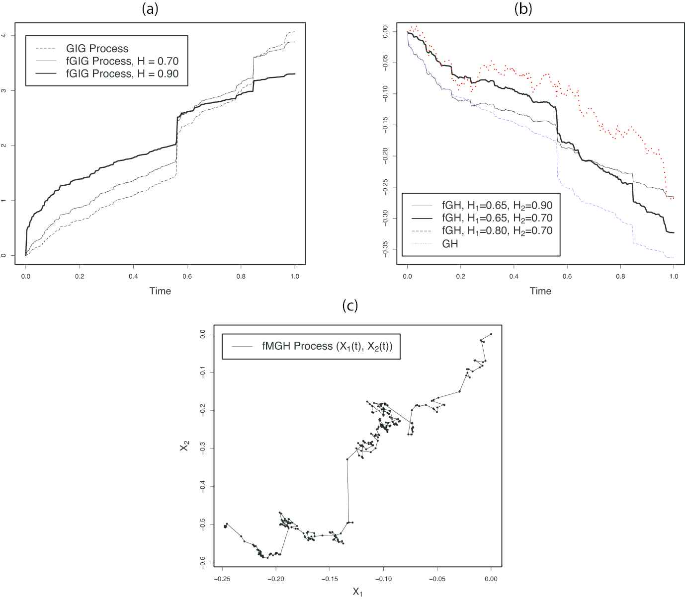
Figure 1 illustrates the simulated sample paths from a Generalized Inverse Gaussian process with M=250 and parameters λ=−1.2, δ=0.1, and γ=0.01. The GIG process on panel (a) depicts a sample path from the Generalized Inverse Gaussian process. Then, obtained are the fGIGs, the fractional Generalized Inverse Gaussian processes, with H=0.70 and 0.90 from the GIG process. Panel (b) gives the simulated sample paths of the univariate fractional Generalized Hyperbolic processes with β=−0.05, comparing with the path of the nonfractional Generalized Hyperbolic process. Notice that the sample paths for the fractional processes have less fluctuations than the path for nonfractional process, indicating the persistence of long-range dependence property of the fractional Generalized Hyperbolic processes. In panel (c), the two-dimensional plot for the bivariate fractional Generalized Hyperbolic process is presented using Equation (7) with H1=0.55, H2=0.80, β=(−0.05,−0.03)T, and Cov(BH1,1(1),BH1,2(1))=0.75.
Figure 1
Sample Paths from Simulations (a) Sample Paths for (Fractional) Generalized Inverse Gaussian Processes (b) Sample Paths for (Fractional) Generalized Hyperbolic Processes (c) Sample Path for Fractional Bivariate Generalized Hyperbolic Process.
7. CONCLUDING REMARKS
In this paper, a fractional Generalized Hyperbolic process defined by the time-changed fractional Brownian motion with the fractional Generalized Inverse Gaussian process is presented. This process is featured by the capability to capture not only the endogenous long-range dependence by the fractional Brownian motion, but also the exogenous long-range dependence by the fractional Generalized Inverse Gaussian process. That is, the process could implement the long-range dependence in volatility as well as the long-range dependence in random process itself.
CONFLICTS OF INTEREST
All authors report no conflicts of interest relevant to this article.
AUTHORS' CONTRIBUTIONS
We thank the anonymous reviewers for helpful comments on earlier drafts of the manuscript.
TY  - JOUR
AU  - Sung Ik Kim
AU  - Young Shin Kim
PY  - 2020
DA  - 2020/10/06
TI  - A New Stochastic Process with Long-Range Dependence
JO  - Journal of Statistical Theory and Applications
SP  - 432
EP  - 438
VL  - 19
IS  - 3
SN  - 2214-1766
UR  - https://doi.org/10.2991/jsta.d.200923.001
DO  - 10.2991/jsta.d.200923.001
ID  - Kim2020
ER  -

 , Young Shin Kim2