
A Note on Topp-Leone Odd Log-Logistic Inverse Exponential Distribution
- DOI
- 10.2991/jsta.d.200827.002How to use a DOI?
- Keywords
- Inverse exponential distribution; Topp-Leone odd log-logistic family; Hazard function; Residual and reversed residual life functions; Unimodal
- Abstract
The inverse exponential distribution is widely used in the field of reliability. In this article, we present a generalization of the inverse exponential distribution in formation of Topp-Leone odd log-logistic inverse exponential distribution. We provide a comprehensive account of some mathematical properties of the Topp-Leone odd log-logistic inverse exponential distribution. The possible shapes of the corresponding probability density function and hazard function are obtained and graphical demonstration are presented. The distribution is found to be unimodal. The results for moment, moment-generating function, and probability-generating function are computed. The residual and reversed residual functions are also obtained. The proposed method of maximum likelihood is used for the estimation of model parameters. The performance of the parameters is investigated through simulation. The usefulness of the proposed model is illustrated by means of a real data set.
- Copyright
- © 2020 The Authors. Published by Atlantis Press B.V.
- Open Access
- This is an open access article distributed under the CC BY-NC 4.0 license (http://creativecommons.org/licenses/by-nc/4.0/).
1. INTRODUCTION
Keller and Kamath [1] introduced the inverse exponential (IEx) distribution to study the reliability of computer control (CNC) machine tools. Lin et al. [2] discussed the IEx distribution in term of different causes of failure for the machines. They obtained the maximum likelihood estimator and confidence limits for the parameter and the reliability function using complete samples. They also compared this model with the inverted Gaussian and log-normal distributions based on a maintenance data set. Sanku Dey [3] and Gyan Prakash [4] studied the IEx distribution according to Bayesian point of view. Abouammoh and Alshingiti [5] worked on the addition of an extra shape parameter to obtain the generalized IEx distribution. It is to be noted that this distribution originated from the exponentiated Frechet distribution studied by Nadarajah and Kotz [6].
Several interesting generalizations of the IEx distribution have been derived including transmuted-generalized IEx distribution by Elbatal [7], the Kumaraswamy IEx distribution by Oguntunde et al. [8], the transmuted IEx distribution by Oguntunde and Adejumo [9], the exponentiated-generalized IEx distribution by Oguntunde et al. [10], and the beta-generalized IEx distribution by Bakoban and Abu-Zinadah [11].
The most common exhibition of hazard rates appeared in practice is the bathtub shaped. A simple model form bathtub-shaped hazard rates is the Topp-Leone distribution introduced by Topp and Leone [12]. The quantile function of this model has closed-form and the model is also very flexible to generate the data.
We start by defining the class of probability distribution introduced by Alizadeh et al. [13] using the cumulative distribution function (cdf) of the odd log-logistic (OLL) distribution as a generator and named as the Topp-Leone odd log-logistic (TLOLL-G) family of distributions. The proposed family has two additional shape parameters. The distribution function (cdf) of the proposed class of distributions is given as follows:
In this study, we introduce a generalization of the IEx distribution named as the Topp-Leone odd log-logistic inverse exponential (TLOLL-IEx) distribution. The motivation of this generalization of IEx distribution is to enhance its applicability and adaptability. The addition of two shape parameters makes it more compatible for modeling the real life scenarios.
The organization of this article is as follows: The proposed TLOLL-IEx distribution and its properties are given in Section 2. Estimation of the model parameters is computed in Section 3. The performance of the parameters is investigated through simulation in Section 4. The application of the proposed model is illustrated in Section 5. The discussion ends with some concluding remarks in Section 6.
2. TOLL-IEx DISTRIBUTION AND ITS PROPERTIES
In this section, we derive the density function of the TLOLL-IEx distribution. For this aim, we consider the cdf of IEx distribution as
Using (2.1) in (1.1), we have the cdf of TLOLL-IEx distribution as
The corresponding density of the TLOLL-IEx distribution is obtained by differentiating Eq. (2.3) and given as
We study some useful and important properties of the new distribution. The distributional properties of the proposed distribution is obtained for real values of
2.1. Shape
The density function TLOLL-IEx distribution as form (2.4) is given as
For real
Then, the pdf of TLOLL-IEx distribution is written as
Here,
We define
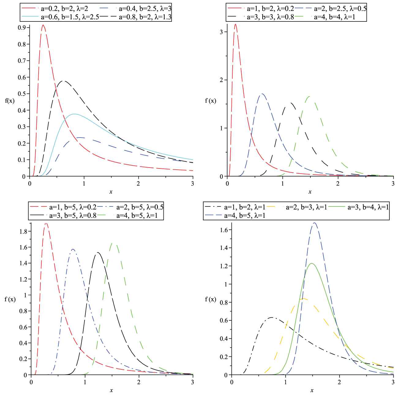
The density function for the Topp-Leone odd log-logistic inverse exponential (TLOLL-IEx) distribution for several values of parameters.
Quantile Function and Various Relevant Measures
The quantile function of TLOLL-IE distribution corresponding to (2.1) is given by
The above expression concede us to extract the following form of statistical measures for the proposed model i. The first quartile Q1, the second quartile Q2(median), and the third quartile Q3 of the TLOLL-IE distribution correspond to the values u = 0.25, 0.50, and 0.75, respectively. ii. The skewness and kurtosis can be calculated by using the following relations, respectively. Bowleys skewness is based on quartiles in Kenney and Keeping (1962) calculated by
Moors kurtosis (Moors, 1988) is based on octiles via the form
Asymptotics
Corollary 3.1:
Let
Corollary 3.2:
The asymptotics of
2.2. Moment
The
One can see, (2.6) is an infinite weighted sum of moments of the IEx distribution. The higher-order moments can be obtained by substituting
2.3. Moment-Generating Function and Probability-Generating Function
The moment-generating function (mgf) of the TLOLL-IEx distribution is obtained by
Similarly, the probability-generating function (pgf) of the TLOLL-IEx distribution is defined as follows:
Some reliability measure including hazard rate function also known as reliability function
2.4. Hazard Function
The hazard function for any probability distribution is given as
For TLLOL-IE distribution, the hazard function is obtained by
Figure 2 presents, the plots of the hazard function for TLOLL-IEx distribution with several values of parameters. As seen in Figure 2, the hazard function of the TLOLL-IEx distribution is very flexible. The reversed hazard function is obtained as follows:
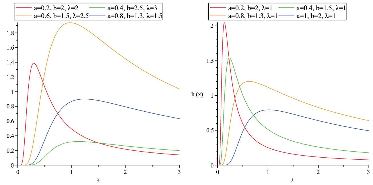
Plots for the hazard function of Topp-Leone odd log-logistic inverse exponential (TLOLL-IEx) distribution for several values of parameters.
2.5. Moments for Residual and Reversed Residual Life
The
The mean residual life of
The
3. INFERENCE
In this section, the method of maximum likelihood is considered for the estimation of parameters of TLOLL-IEx distribution. Let,
We can maximize the above equation using R (optim function), SAS (PROCNLMIXED), and Ox program (MaxBFGS sub-routine) or by solving the nonlinear likelihood equations by differentiation. The score vector components, say
Here,
By determining the inverse dispersion matrix, the asymptotic variances and covariances of the MLEs for
4. SIMULATION STUDY
In this section, we conduct a simulation study. We generate 10,000 samples of size, n = 50, 100, 250, 500 and n = 1000 of the TLOLL-IEx model. The evaluation of estimates is based on the mean, the mean squared error (MSE), and We use R software for computation. The results in Table 1 show that the estimates are closer to the true values of the parameters from all sample size which clearly indicates that estimate are quite suitable. As the value of
| Mean |
MSE |
AL |
|||||||||
|---|---|---|---|---|---|---|---|---|---|---|---|
| 50 | 0.661 | 1.321 | 0.783 | 0.312 | 0.215 | 1.315 | 0.831 | 0.737 | 0.749 | ||
| 100 | 0.601 | 1.135 | 0.632 | 0.234 | 0.177 | 1.103 | 0.557 | 0.811 | 0.861 | ||
| 0.5 | 0.5 | 250 | 0.549 | 1.075 | 0.554 | 0.133 | 0.121 | 0.311 | 0.313 | 0.853 | 0.882 |
| 500 | 0.531 | 1.041 | 0.516 | 0.031 | 0.037 | 0.108 | 0.104 | 0.873 | 0.931 | ||
| 1000 | 0.503 | 1.009 | 0.505 | 0.011 | 0.015 | 0.036 | 0.023 | 0.941 | 0.953 | ||
| 50 | 0.537 | 1.319 | 2.417 | 0.578 | 0.315 | 2.112 | 1.731 | 0.821 | 0.886 | ||
| 100 | 0.522 | 1.217 | 2.313 | 0.441 | 0.257 | 1.011 | 1.335 | 0.851 | 0.922 | ||
| 0.5 | 2 | 250 | 0.519 | 1.033 | 2.139 | 0.361 | 0.113 | 0.713 | 0.716 | 0.885 | 0.936 |
| 500 | 0.509 | 1.015 | 2.101 | 0.131 | 0.057 | 0.317 | 0.318 | 0.911 | 0.948 | ||
| 1000 | 0.501 | 1.003 | 2.011 | 0.053 | 0.013 | 0.103 | 0.107 | 0.942 | 0.953 | ||
| 50 | 0.631 | 1.353 | 1.619 | 0.485 | 0.553 | 0.972 | 2.538 | 0.831 | 0.841 | ||
| 100 | 0.539 | 1.172 | 1.761 | 0.349 | 0.331 | 0.609 | 1.549 | 0.866 | 0.883 | ||
| 3 | 2.5 | 250 | 0.526 | 1.105 | 1.837 | 0.111 | 0.145 | 0.363 | 0.649 | 0.913 | 0.914 |
| 500 | 0.513 | 1.051 | 1.935 | 0.018 | 0.051 | 0.131 | 0.341 | 0.937 | 0.938 | ||
| 1000 | 0.501 | 1.011 | 1.992 | 0.001 | 0.012 | 0.015 | 0.131 | 0.944 | 0.948 | ||
Estimated biases, mean squared errors (MSEs), average lenghts(ALS) for the several parameter values.
5. APPLICATION
In this part, we discuss the applicability of TLOLL-IEx model in real-life phenomena. We consider the data of the tensile strength, measured in GPa, of 69 carbon fibers tested under tension at gauge lengths of 20 mm given by Chwastiak
| 1.312, 1.314, 1.479, 1.552, 1.700, 1.803, 1.861, 1.865, 1.944, 1.958, 1.966, 1.997, 2.006, |
| 2.021, 2.027, 2.055, 2.063, 2.098, 2.140, 2.179, 2.224, 2.240, 2.253, 2.270, 2.272, 2.274, |
| 2.301, 2.301, 2.359, 2.382, 2.382, 2.426, 2.434, 2.435, 2.478, 2.490, 2.511, 2.514, 2.535, |
| 2.554, 2.566, 2.570, 2.586, 2.629, 2.633, 2.642, 2.648, 2.684, 2.697, 2.726, 2.770, 2.773, |
| 2.800, 2.809, 2.818, 2.821, 2.848, 2.880, 2.954, 3.012, 3.067, 3.084, 3.090, 3.096, 3.128, |
| 3.233, 3.433, 3.585, 3.585 |
Carbon fiber data.
| Distribution | Abbreviation | References |
|---|---|---|
| Topp-Leone OLL IEx | TLOLL-IEx | Proposed |
| IEx | IE | [7] |
| Exponential | E | [15] |
| Lindley | L | [9] |
| Generalized Lindley | GL | [9] |
| Generalized Gamma | GG | [9] |
| Exponential Power | EP | [15] |
| Power Quasi Lindley | PQL | [16] |
| Weibull | W | [17] |
| Sujatha | S | [10] |
| Generalized Sujatha | GS | [10] |
Fitted distributions and their abbreviations.
The unknown parameters of each distribution are estimated using the maximum likelihood method.
| Distribution | Estimated Parameters | AIC | CAIC | BIC | ||
|---|---|---|---|---|---|---|
| TLOLL( |
6.4855 | 0.5668 | 2.0404 | 103.8239 | 104.1931 | 110.5262 |
| IE( |
2.343 | 264.0296 | 264.0893 | 266.2637 | ||
| E( |
2.4513 | 263.7352 | 263.7949 | 265.9693 | ||
| L( |
0.6545 | 240.3805 | 240.4402 | 242.6146 | ||
| GL( |
9.3907 | 22.7198 | 4.771 | 106.0848 | 106.454 | 112.7871 |
| GG( |
3.5861 | 2.6483 | 0.3044 | 103.9877 | 104.3569 | 110.69 |
| EP( |
2.992 | 3.7061 | 111.204 | 111.3858 | 115.6722 | |
| W( |
3.843 | 0.088 | 275.8682 | 276.05 | 280.3364 | |
| S( |
0.0956 | 243.5 | 243.63 | 244.93 | ||
| GS( |
0.0972 | 14.473 | 244.54 | 244.68 | 243.97 | |
MLE, maximum likelihood estimation; AIC, Akaike information criterion; CAIC, consistent Akaike information criterion; BIC, Bayesian information criterion.
Estimated parameter values are obtained from related references.
MLEs and the values of AIC, CAIC, and BIC statistics.
We also obtain a visual comment with histogram given in Figure 3 for the best model.
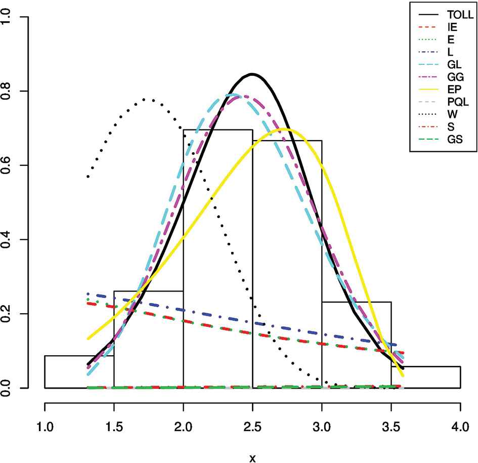
Graph for fitted distributions to the data set.
6. CONCLUSION
In this paper, the discussion has been carried out through the generalization of the IEx distribution. We motivate from the TLOLL family of distributions and named the proposed model as TLOLL-IEx distribution. Several structural characteristics of the proposed distribution are derived and discussed. The maximum likelihood method is employed for estimating the model parameters. For effectiveness of the derived model, we consider a real-life data set and the results are compared with some well-known existing distributions. The TLOLL-IEx distribution is found unimodal. We hope that this generalization will applicable in the fields of reliability and lifetime analysis.
CONFLICTS OF INTEREST
The authors declare no potential conflict of interests.
AUTHORS' CONTRIBUTIONS
All authors contributes equally.
ACKNOWLEDGMENTS
We are very thankful to all referees for their precious time for the evaluation of the article. We also appreciate the correspondence of the editor.
REFERENCES
Cite this article
TY  - JOUR
AU  - Salman Abbas
AU  - Fakhar Mustafa
AU  - Syed Ali Taqi
AU  - Selen Cakmakyapan
AU  - Gamze Ozel
PY  - 2020
DA  - 2020/09/07
TI  - A Note on Topp-Leone Odd Log-Logistic Inverse Exponential Distribution
JO  - Journal of Statistical Theory and Applications
SP  - 397
EP  - 407
VL  - 19
IS  - 3
SN  - 2214-1766
UR  - https://doi.org/10.2991/jsta.d.200827.002
DO  - 10.2991/jsta.d.200827.002
ID  - Abbas2020
ER  -