
Behavior of OC Curve of Generalized Exponentiated Data
- DOI
- 10.2991/jsta.d.200714.001How to use a DOI?
- Keywords
- Operating characteristics curve; Generalized exponential distribution; Left censored
- Abstract
In this paper a generalized exponential distribution is considered for analyzing left-censored lifetime data as such mechanisms are applicable when the observations become available in an ordered manner with some cases where the origin and the event both occur prior to the start of follow-up. In the present study a test procedure is developed which will approximate a prescribed operating characteristics curve. We also done testing of hypothesis and tried to find values of r and C subject to the operating characteristics curve be such that
- Copyright
- © 2020 The Authors. Published by Atlantis Press B.V.
- Open Access
- This is an open access article distributed under the CC BY-NC 4.0 license (http://creativecommons.org/licenses/by-nc/4.0/).
1. INTRODUCTION
Two-parameter generalized exponential (GE) distribution was originally introduced by Gupta and Kundu [1] as a skewed distribution, and as an alternative to Weibull, gamma, or log-normal distribution. Because of the shape and scale parameters, it is observed that GE distribution can take different shapes and it can be used quite effectively to analyze skewed data. Extensive work has been done by several authors on GE distribution. See, e.g., by Gupta and Kundu [2–4], Raqab [5], Raqab and Ahsanullah [6], Zheng [7], and Mitra and Kundu [8] studied the maximum likelihood estimators of the unknown parameters of the GE distribution for left-censored data.
GE distribution, which more accurately represents time to failure, is used instead of more commonly used exponential distribution. Although, incorporation of GE distribution in life testing modeling adds to complexity of modeling and estimation, but due to its flexibility, it fits more accurately to life data than exponential distribution.
The two-parameter GE distribution has the following density function:
Cumulative distribution function (cdf)
Reliability function
Hazard function
Here
There is a widespread application and use of left-censoring or left-censored data in survival analysis and reliability theory, in which a subject is left censored if it is known that the event of interest occurs some time before the recorded follow-up period. For example, a study conducts as investigating factors influencing days to first oestrus in dairy cattle. You start observing your population (for argument's sake) at 40 days after calving but find that several cows in the group have already had an oestrus event. These cows are said to be left censored at day 40, in medical studies patients are subject to regular examinations. Discovery of a condition only tells us that the onset of sickness fell in the period since the previous examination and nothing about the exact date of the attack. Thus the time elapsed since onset has been left censored. Similarly, we have to handle left-censored data when estimating functions of exact policy duration without knowing the exact date of policy entry; or when estimating functions of exact age without knowing the exact date of birth. A study on the “Patterns of Health Insurance Coverage among Rural and Urban Children” (Coburn et al. [9]) faces this problem due to the incidence of a higher proportion of rural children whose spells were “left censored” in the sample (i.e., those children who entered the sample uninsured), and who remained uninsured throughout the sample. Yet another study (Danzon et al. [10]) which used data on over 900 firms for the period 1988–2000 to estimate the effect on phase-specific (phases 1, 2 and 3) biotech and pharmaceutical R&D success rates of a firm's overall experience, its experience in the relevant therapeutic category, the diversification of its experience across categories, the industry's experience in the category, and alliances with large and small firms, saw that the data suffered from left censoring. This occurred, e.g., when a phase 2 trial was initiated for a particular indication where there was no information on the phase 1 trial. Application can also be traced in econometric model, e.g., for the joint determination of wages and turnover. Here, after the derivation of the corresponding likelihood function, an appropriate dataset is used for estimation. For a model that is designed for a comprehensive matched employer–employee panel dataset with fairly detailed information on wages, tenure, experience, and a range of other covariates, it may be seen that the raw dataset may contain both completed and uncompleted job spells. A job duration might be incomplete because the beginning of the job spells is not observed, which is an incidence of left censoring (Bagger [11]). For some further examples, one may refer to Balakrishnan and Varadan [12], Lee et al. [13], etc.
Put in general terms, let
The main aim of this paper is to establishing the Cramer Roa lower bound and efficiency of estimates with respect to Cramer Roa lower bound. Besides that we also derived minimum variance of the biased estimates, also established testing of hypothesis and studied behavior of operating characteristics (OC) curve of GE distribution. From the point of view of acceptance testing, the OC curve based on the r out of n ordered observations for left-censored data (acceptance region of the form
2. MAXIMUM LIKELIHOOD ESTIMATION
In this section, maximum likelihood estimators of the
The log likelihood function of the observed sample is
The maximum likelihood estimation (MLE) of
The MLE
Result 1: If
Result 2:
Result 3:
The density (7) depends only on
3. CRAMER RAO LOWER BOUND (CRLB)
Cramer Rao lower bound unbiased, efficient, and sufficient estimate of MLE and unbiased estimate of the parameter
The log likelihood function of the observed sample is
Using Equation (5) or (6) in Equation (9) we have
Therefore
Therefore Cramer Rao Lower Bound is
Efficiency of the estimate
Efficiency of the estimate
Clearly efficiency of
Minimum variance biased estimate of
4. DERIVATION OF TEST BASED ON THE r OUT OF n ORDERED FOLLOW-UP OBSERVATIONS DRAWN FROM GED
In this section we develop a best test on the first r ordered observations (from a sample of size n) so as to decide between two values of
By the best test we mean according to the usual Neyman–Pearson terminology a test which has the property that among all tests having a fixed probability
To derive the best test we use Neyman-Pearson (NP) lemma, according to the lemma a best test must be one for which the region of rejection can be found from the inequality.
Case I: when
Because
Since
Case II when
Since
5. DETERMINATION OF CONSTANTS C1 AND C2
The constants
Case I when
To find
Thus
Let us denote a chi-square variable with n degrees of freedom as
Then (12) can be written as
Hence (12) will be satisfied if the region of rejection for
It is convenient in what follows to use acceptance rather than rejection regions. Consequently the NP theory tells us that a simple test for
Case II when
Thus in a analogue as discussed earlier, the above probability equation can yield
The best critical region can be written in the form as given below
It is convenient in what fallows to use acceptance rather than rejection regions. Consequently the NP theory tells us that a simple test for
6. POWER FUNCTION OF THE TEST
Case I when
According to NP lemma the region of rejection (13) has a greater chance of rejecting
Case II when
According to NP lemma the region of rejection (15) has a greater chance of rejecting
7. OC FUNCTION
Case I when
The graph of
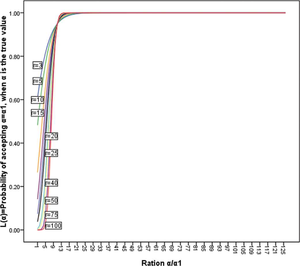
OC of fests of the form
In the problem just discussed, it was assumed that
This implies that
Knowing (19) makes it an easy matter to find that integer r which ensures that the OC curve pass most nearly through the points
This is the value of r which we wish to use. If with this value of r we use an acceptance region
We shall have a test whose OC curve is such that
Case II when
The graph of
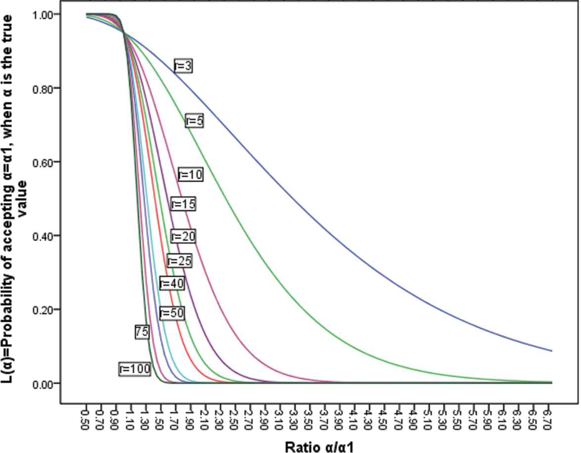
Operating characterstics of tests of the form
In the problem just discussed, it was assumed that
This implies that
Knowing (22) makes it an easy matter to find that integer r which ensures that the OC curve pass most nearly through the points
This is the value of r which we wish to use. If with this value of r we use an acceptance region
We shall have a test whose OC curve is such that
8. UNIFORMLY MOST POWERFUL CRITICAL REGION
Case I: when
The best critical region as given in (13) is
It is independent of
Case II: when
The best critical region as given in (15) is
It is independent of
However, since the two critical regions
If
| α1/α2 | r | C1/α1 | C1*/α1 | R | C1/α1 | C1*/α1 | r | C1/α1 | C1*/α1 |
|---|---|---|---|---|---|---|---|---|---|
| or | Or | or | Or | or | or | or | |||
| C2*/α2 | C2/α2 | C2*/α2 | C2/α2 | C2*/α2 | C2/α2 | ||||
| α = 0.01, β = 0.01 | α = 0.01, β = 0.05 | α = 0.01, β = 0.1 | |||||||
| 1.5 | 132 | 0.82403 | 0.82435 | 95 | 0.797427 | 0.796082 | 76 | 0.777591 | 0.778725 |
| 2 | 45 | 0.725126 | 0.728697 | 32 | 0.686571 | 0.68677 | 25 | 0.656565 | 0.66333 |
| 2.5 | 26 | 0.661445 | 0.665692 | 18 | 0.614133 | 0.61886 | 14 | 0.579971 | 0.591365 |
| 3 | 18 | 0.614133 | 0.623938 | 12 | 0.558402 | 0.577683 | 10 | 0.532393 | 0.535793 |
| 4 | 11 | 0.54605 | 0.576369 | 8 | 0.500001 | 0.502409 | 6 | 0.457719 | 0.475904 |
| 5 | 8 | 0.500001 | 0.550565 | 6 | 0.457719 | 0.45924 | 4 | 0.398203 | 0.458513 |
| 10 | 4 | 0.398203 | 0.48588 | 3 | 0.35689 | 0.366887 | 2 | 0.30128 | 0.376073 |
| 15 | 3 | 0.35689 | 0.458668 | 2 | 0.30128 | 0.375205 | 2 | 0.30128 | 0.250715 |
| 20 | 2 | 0.30128 | 0.673153 | 2 | 0.30128 | 0.281404 | 2 | 0.30128 | 0.188037 |
| α = 0.05, β = 0.01 | α = 0.05, β = 0.05 | α = 0.05, β = 0.1 | |||||||
| 1.5 | 98 | 0.853424 | 0.854591 | 66 | 0.825963 | 0.826612 | 51 | 0.805852 | 0.807819 |
| 2 | 34 | 0.770537 | 0.775582 | 22 | 0.727503 | 0.738565 | 17 | 0.699554 | 0.709745 |
| 2.5 | 20 | 0.71738 | 0.721883 | 13 | 0.668636 | 0.67624 | 10 | 0.636731 | 0.642952 |
| 3 | 14 | 0.677357 | 0.68806 | 9 | 0.6235 | 0.638947 | 7 | 0.591097 | 0.599094 |
| 4 | 9 | 0.6235 | 0.641491 | 6 | 0.57072 | 0.57405 | 4 | 0.515886 | 0.573142 |
| 5 | 7 | 0.591097 | 0.600804 | 4 | 0.515886 | 0.585515 | 3 | 0.476509 | 0.544432 |
| 10 | 3 | 0.476509 | 0.688002 | 2 | 0.421597 | 0.562807 | 2 | 0.421597 | 0.376073 |
| 15 | 2 | 0.421597 | 0.897537 | 2 | 0.421597 | 0.375205 | 2 | 0.421597 | 0.250715 |
| 20 | 2 | 0.421597 | 0.673153 | 2 | 0.421597 | 0.281404 | 2 | 0.421597 | 0.188037 |
| α = 0.1, β = 0.01 | α = 0.1, β = 0.05 | α = 0.1, β = 0.1 | |||||||
| 1.5 | 82 | 0.87422 | 0.875869 | 53 | 0.84776 | 0.539311 | 40 | 0.828344 | 0.829731 |
| 2 | 29 | 0.803771 | 0.807497 | 18 | 0.762515 | 0.352952 | 14 | 0.738476 | 0.739206 |
| 2.5 | 17 | 0.757185 | 0.764511 | 10 | 0.703928 | 0.254692 | 8 | 0.679641 | 0.687268 |
| 3 | 12 | 0.722973 | 0.736895 | 7 | 0.664637 | 0.197032 | 5 | 0.625501 | 0.685141 |
| 4 | 8 | 0.679641 | 0.688206 | 5 | 0.625501 | 0.13656 | 3 | 0.563664 | 0.68054 |
| 5 | 6 | 0.646923 | 0.672162 | 3 | 0.563664 | 0.095302 | 2 | 0.514176 | 0.752146 |
| 10 | 3 | 0.563664 | 0.688002 | 2 | 0.514176 | 0.04216 | 2 | 0.514176 | 0.376073 |
| 15 | 2 | 0.514176 | 0.897537 | 2 | 0.514176 | 0.028106 | 2 | 0.514176 | 0.250715 |
| 20 | 2 | 0.514176 | 0.673153 | 2 | 0.514176 | 0.02108 | 2 | 0.514176 | 0.188037 |
Values of
ACKNOWLEDGEMENTS
The authors appreciate and thank the referee and the editor for many helpful comments and suggestions, which substantially simplified the paper.
REFERENCES
Cite this article
TY  - JOUR
AU  - Anwar Hassan
AU  - Mehraj Ahmad
AU  - Najmus Saquib Hassan
PY  - 2020
DA  - 2020/07/21
TI  - Behavior of OC Curve of Generalized Exponentiated Data
JO  - Journal of Statistical Theory and Applications
SP  - 332
EP  - 341
VL  - 19
IS  - 2
SN  - 2214-1766
UR  - https://doi.org/10.2991/jsta.d.200714.001
DO  - 10.2991/jsta.d.200714.001
ID  - Hassan2020
ER  -