Odd ratio function; Order statistics; Bootstrap; Lindley distribution; Characterizations
Abstract
In the present paper, a new family of lifetime distributions is introduced via odd ratio function, the well-known concept in survival analysis and reliability engineering. Some important properties of the proposed model including survival function, quantile function, hazard function, order statistic are obtained in a general setting. A special case of this new family is taken up by considering exponential and Lindley models as the parent distributions. In addition, estimation of the unknown parameters of the special model will be examined from the perspective of the classic statistics. A simulation study is presented to investigate the bias and mean square error of the maximum likelihood estimators. Moreover, an example of real data set is studied; point and interval estimations of all parameters are obtained by maximum likelihood and bootstrap (parametric and non-parametric) procedures. Finally, the superiority of the proposed model in terms of the parent exponential distribution over other fundamental statistical distributions is shown via the example of real observations.
The statistical distribution theory has been widely explored by researchers in recent years. Given the fact that the data from our surrounding environment follow various statistical models, it is necessary to extract and develop appropriate high-quality models.
Recently, Alzaatreh et al. [2] have introduced a new model of lifetime distributions, which the researchers refer to its especial case as odd−G distribution. It is based on the combination of an arbitrary cumulative distribution function CDF with odd ratio of the baseline CDF as G. The integration form of the new CDF is
Hx=∫−∞Gx1−Gxftdt,
where f is the probability density function PDF of arbitrary CDF. This interesting method attracted the attention of some researchers. We refer the reader to [4,1,8,9,14]. Generating new model based on this method resulted in creating very flexible statistical model.
In the present paper, we introduce a new family of lifetime distributions based on the odd ratio of a parent distribution G for general hyperbolic cosine-F HCF family of lifetime distributions that recently proposed by Kharazmi and Saadatinik [7]. This new model will be denoted by odd−HCF−Gor OHCFG distribution. One of our main motivation to introduce this new category of distributions is to provide more flexibility for fitting real datasets compare to other well-known classic statistical distributions.
In summary, we first obtain the fundamental and statistical properties of the OHCFG in general setting and then we propose a special case of this model by considering exponential distributions in place of the parent distribution F and Lindley distribution instead of the parent distribution G. It is referred to as Odd Hyperbolic Cosine Exponential Lindley (OHCEL) distribution. We provide a comprehensive discussion about statistical and reliability properties of new OHCEL model. Furthermore, we consider maximum likelihood and bootstrap estimation procedures in order to estimate the unknown parameters of the new model for a complete data set. In addition, parametric and non-parametric bootstrap CIs are calculated.
The rest of the paper organized as follows. In the Section 2, a new category of lifetime distributions is introduced based on the fundamental odd quantity and then the main statistical and reliability properties are obtained in general setting. In Section 3, by considering the two exponential and Lindley distributions as the base distributions, a new model is presented according to the general model discussed in Section 1 and its prominent characteristics are studied. This new model refer to as OHCEL distribution. In Section 4, we examine the inferential procedures for estimation unknown parameters of the OHCEL model. In this section, we provide discussions about the maximum likelihood and bootstrap procedures. Applications and numerical analysis of three real data sets are presented in Section 5. Finally, in Section 6 the paper is concluded.
2. NEW GENERAL MODEL AND ITS PROPERTIES
In this section, we provide the structure of our new model and some main properties of the proposed model in general setting. Motivated by idea of Alzaatreh et al. [2], a new class of statistical distributions is proposed. The new model is constructed by applying Alzaattreh idea to the HCF family of lifetime distributions that recently have seen proposed by Kharazmi and Saadatinik [7]. According to Kharazmi and Saadatinik [7] a random variable X has a HCF distribution if its CDF is given by
Hence, if the baseline F and G distributions are invertible then we can easily generate random samples from the OHCFG distribution.
3. OHCEL DISTRIBUTION AS A SPECIAL CASE OF OHCFG MODEL
In this section, we specialize previous mentioned general model by choosing special cases for baseline distributions F and G. We apply the OHCFG method to a specific case of baseline distributions, namely to an exponential distribution and a Lindley distribution and call this proposed model, three-parameter OHCEL distribution.
Definition.
A random variable X has OHCELa,λ,β distribution, if its PDF is given by
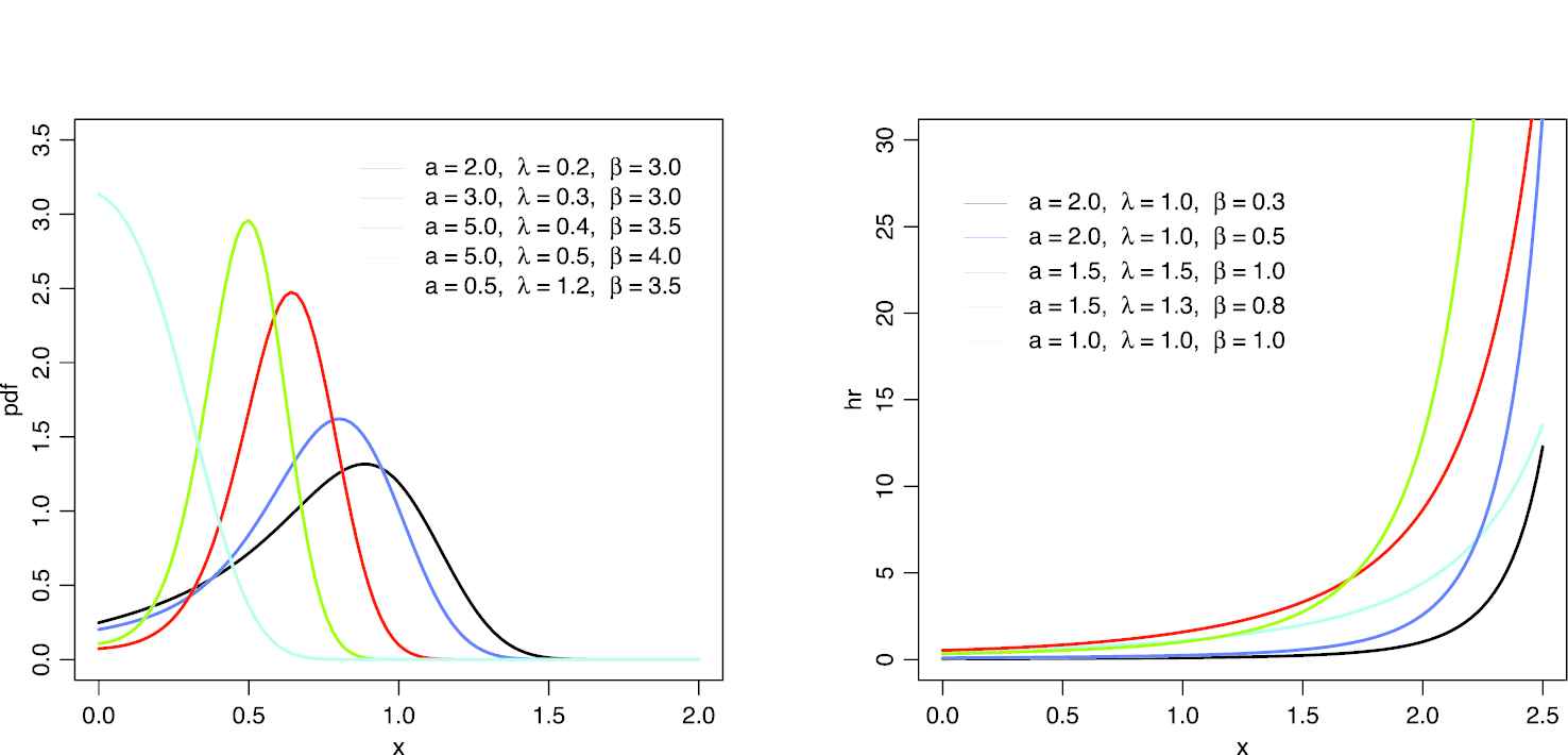
respectively. Some shapes of PDF and hazard function for the selected values of parameters are given in Figures 1 and 2.
Figure 1
Plots of the OHCEL (α, λ, β) (left) and failure rate function (right) for selected values of α, λ, β.
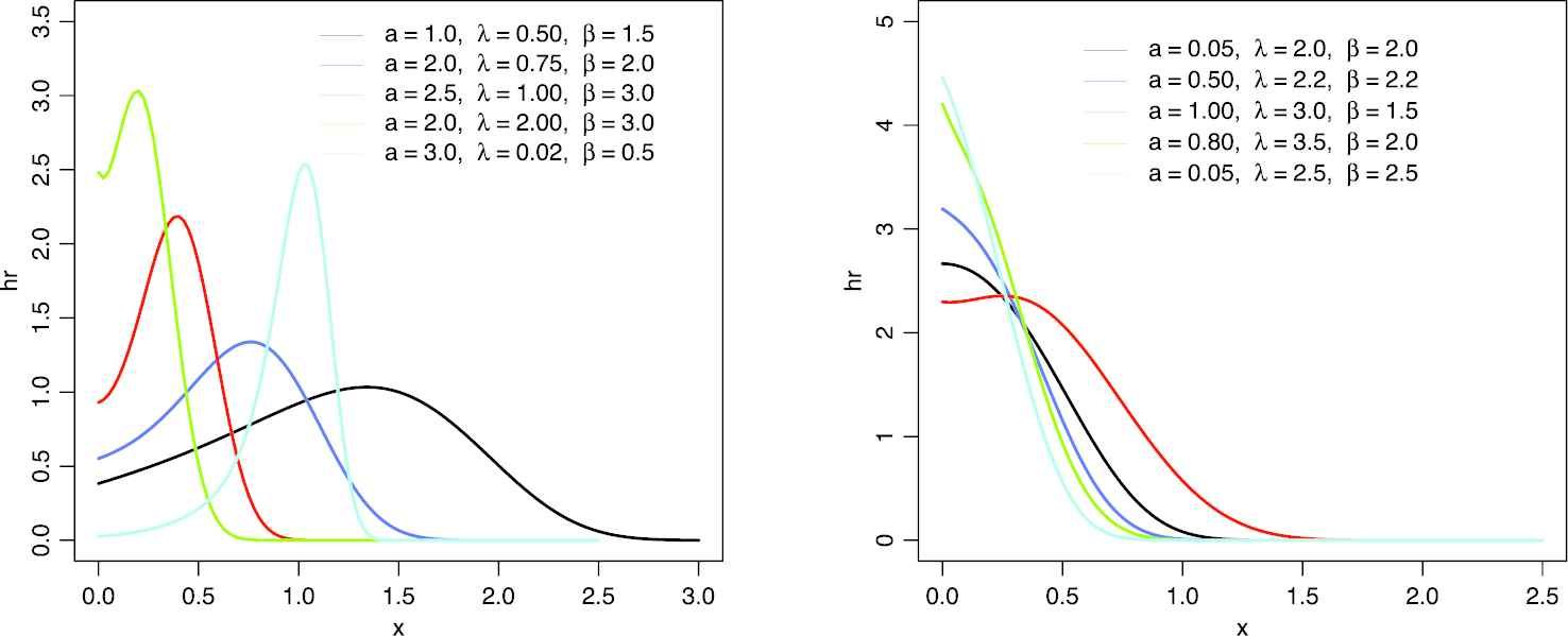
Figure 2
Failure rate function shapes for selected values of the parameters.
3.1. Some Properties of the OHCEL Distribution
In this section, we obtain some properties of the OHCEL distribution, involving quantiles, moments, moment generating function and order statistics distribution. The characterizations of OHCEL distribution are presented in Subsection 3.5.
3.2. Quantiles
For the OHCEL distribution, the pth quantile xp is the solution of Hxp=p, hence
which is the base of generating OHCEL random variates, where W−1 denotes the negative branch of the Lambert function.
3.3. Moments and Moment Generating Function
In this subsection, moments and related measures including coefficients of variation, skewness and kurtosis are presented. Tables of values for the first six moments, standard deviation SD, coefficient of variation CV, coefficient of skewness CS and coefficient of kurtosis CK are also presented. The rth moment of the OHCEL distribution, denoted by μr′, is
where XL∼Lindleyβ and EXL[Xr+t+l]=(r+t+l)!(β+r+t+l+1)βr+l+t(β+1).
The variance, CV, CS, and CK are given by
σ2=μ2′−μ2,CV=σμ=μ2′−μ2μ=μ2′μ2−1,
CS=E[X−μ3][EX−μ2]3∕2=μ3′−3μμ2′+2μ3μ2′−μ23∕2,
and
CK=E[X−μ4][EX−μ2]2=μ4′−4μμ3′+6μ2μ2′−3μ4μ2′−μ22,
respectively.
In the next, we show that the rth moment can be calculated numerically in terms of the selection of different values of the parameters. Table 1 lists the first six moments of the OHCEL distribution for selected values of the parameters, when a=2. Table 2 lists the first six moments of the OHCEL distribution for selected values of the parameters, when β=0.5. These values can be determined numerically using R.
μr′
λ=0.5,β=0.5
λ=0.5,β=1
λ=1.5,β=0.5
λ=1.5,β=1
μ1′
3.941234
1.776483
2.252314
0.9715466
μ2′
18.52086
3.837182
6.5022
1.248397
μ3′
95.44743
9.157249
21.37342
1.850604
μ4′
523.8631
23.37855
76.7875
3.022521
μ5′
3017.057
62.83307
295.3096
5.314822
μ6′
18070.29
176.066
1200.363
9.921312
SD
1.728447
0.8254029
1.195526
0.5518099
CV
0.4385548
0.4646275
0.530799
0.5679706
CS
−0.2124006
−0.1423441
0.1697464
0.2741677
CK
2.401186
2.342314
2.416298
2.459799
CK, coefficient of kurtosis; CS, coefficient of skewness; CV, coefficient of variation; SD, standard deviation.
Table 1
Moments of the OHCEL distribution for selected parameter values when a=2.
μr′
a=0.3,λ=0.5
a=0.5,λ=1
a=0.8,λ=1.2
a=1,λ=1.8
μ1′
3.247616
2.291018
2.13056
1.718264
μ2′
13.50444
7.099715
6.173539
4.117847
μ3′
63.89187
25.72169
20.95563
11.70906
μ4′
329.3444
103.3036
78.96134
37.28532
μ5′
1808.908
447.6086
321.3765
129.1265
μ6′
10444.89
2058.578
1389.934
477.896
SD
1.719718
1.360497
1.278379
1.079544
CV
0.5295325
0.5938394
0.6000202
0.6282761
CS
0.1622998
0.3871795
0.4014882
0.49958
CK
2.312932
2.489167
2.507828
2.653294
CK, coefficient of kurtosis; CS, coefficient of skewness; CV, coefficient of variation; SD, standard deviation.
Table 2
Moments of the OHCEL distribution for selected parameter values when β=0.5.
The moment generating function of the OHCEL distribution is given by
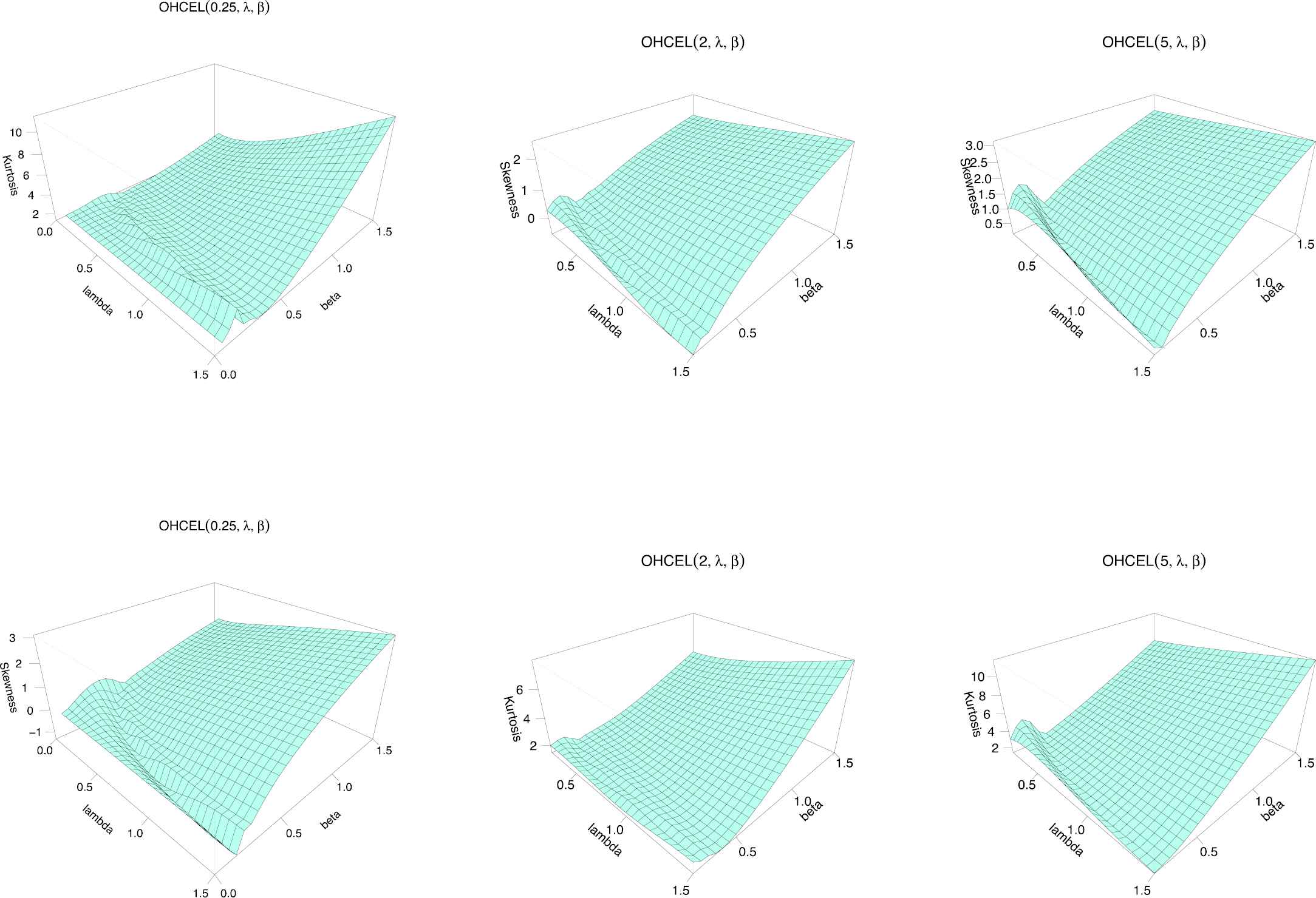
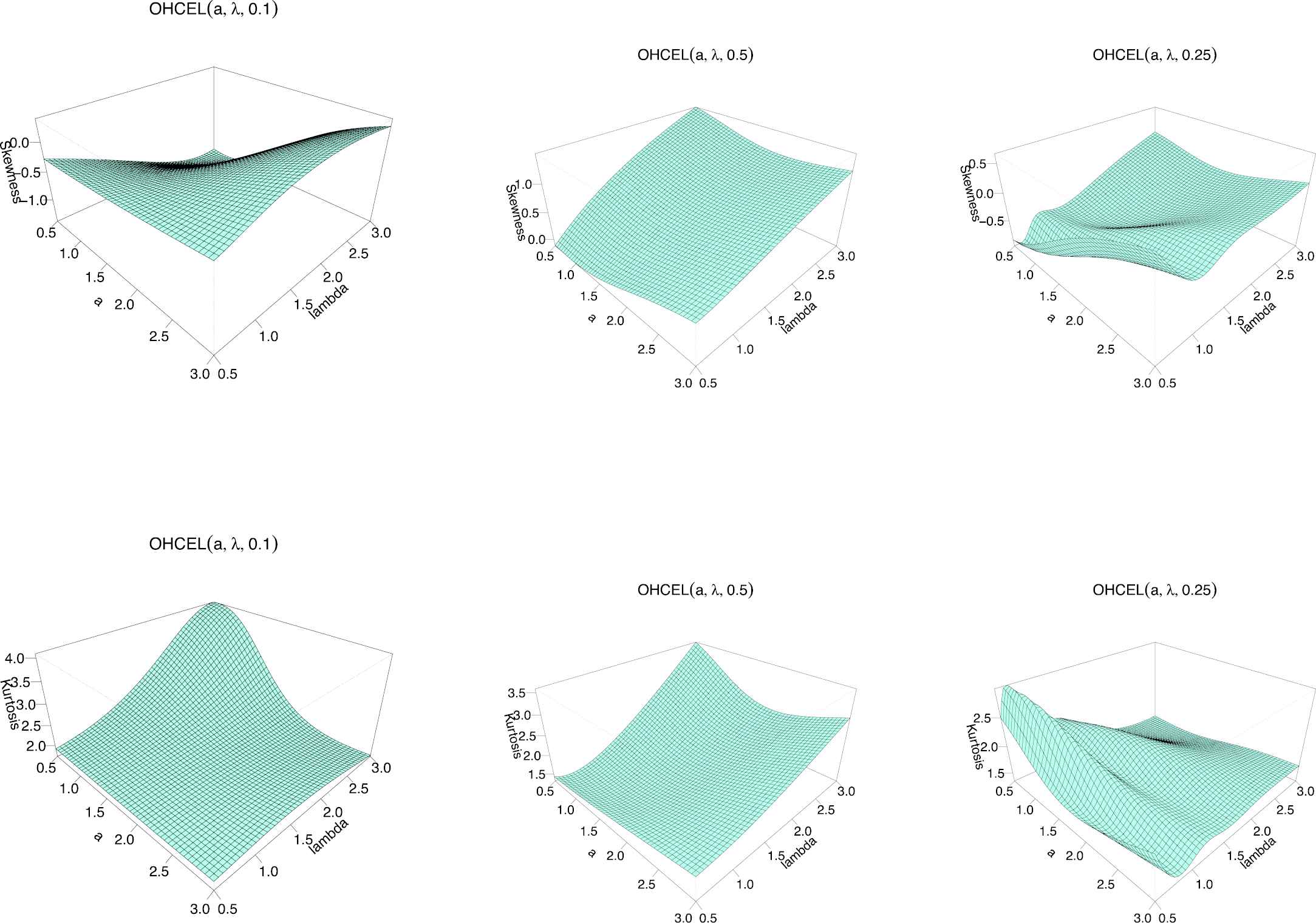
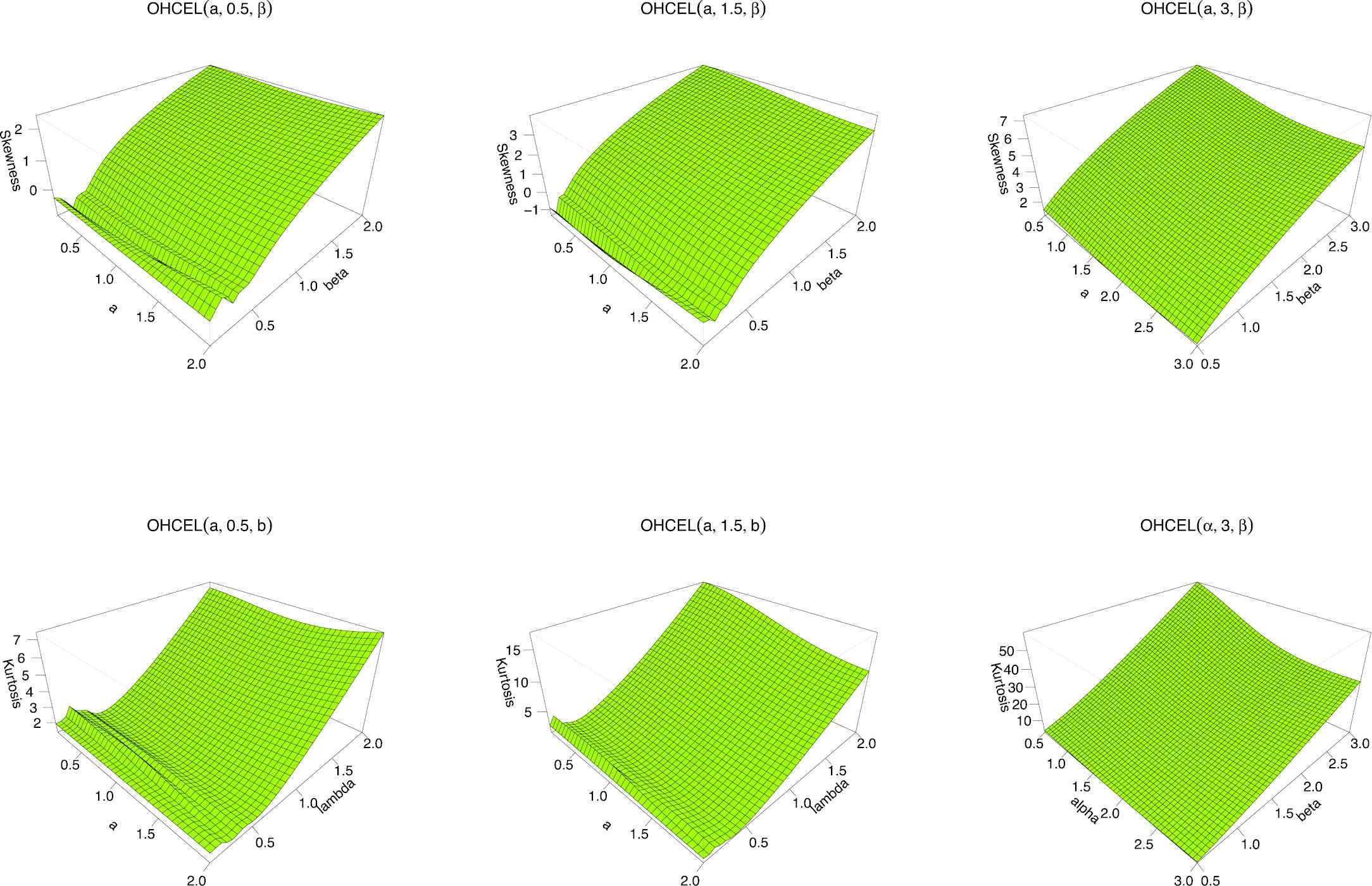
In order to investigate and analyze amount of skewness and kurtosis of the new model under the three parameters a, β and λ, 3D diagrams are presented in Figures 3–5. Analysis of theses graphs shows that all three parameter are effective in variation of skewness and kurtosis.
Figure 3
3D plots of skewness and kurtosis of OHCEL distribution for some fixed values of parameter α.
Figure 4
3D plots of skewness and kurtosis of OHCEL distribution for some fixed values of parameter β.
Figure 5
3D plots of skewness and kurtosis of OHCEL distribution for some fixed values of parameter λ.
3.4. Order Statistics
Order statistics play an important role in probability and statistics. In this subsection, we present the distribution of the ith order statistic from the OHCEL distribution. The PDF of the ith order statistic from the OHCELPDF, fOHCELx, is given by
Using the binomial expansion 1−FOHCELxn−i=∑m=0n−in−im−1mFOHCELxm, we have
fi:nx=1Bi,n−i+1∑m=0n−in−im−1mFOHCELxm+i−1fOHCELx.
3.5. Characterization Results
This section is devoted to the characterizations of the OHCEL distribution based on the ratio of two truncated moments. Note that our characterizations can be employed also when the CDF does not have a closed form. We would also like to mention that due to the nature of OHCEL distribution, our characterizations may be the only possible ones. Our first characterization employs a theorem due to Glänzel [6]. The result, however, holds also when the interval H is not closed, since the condition of the Theorem is on the interior of H.
Proposition 3.5.1.
Let X:Ω→0,∞ be a continuous random variable and let q1(x)=[cosh(a(1−e−λ(1+β1+β+βxeβx−1)))]−1 and q2(x)=q1(x)e−λ(1+β1+β+βxeβx−1) for x>0. The random variable X has PDF (6) if and only if the function η defined in Theorem 1 Glänzel [6] is of the form
Let X:Ω→0,∞ be a continuous random variable and let q1x be as in Proposition 3.5.1. The random variable X has PDF (6) if and only if there exist functions q2 and η defined in Theorem 1 satisfying the following differential equation
where D is a constant. We like to point out that one set of functions satisfying the above differential equation is given in Proposition 3.5.1 with D=0. Clearly, there are other triplets q1,q2,η which satisfy conditions of Theorem 1.
4. INFERNCE PROCEDURE
In this section, we consider estimation of the unknown parameters of the OHCELa,λ,β distribution via maximum likelihood method and bootstrap estimation.
4.1. Maximum Likelihood Estimation
Let x1,…,xn be a random sample from the OHCEL distribution and Δ=a,λ,β be the vector of parameters. The log-likelihood function is given by
The maximum likelihood estimate, Δ̂ of Δ=a,λ,β is obtained by solving the nonlinear equations dLda=0,dLdλ=0,dLdβ=0. These equations are not in closed form and the values of the parameters a, λ and β must be found using iterative methods. Therefore, the maximum likelihood estimate, Δ̂ of Δ=a,λ,β can be determined using an iterative method such as the Newton–Raphson procedure.
4.2. Bootstrap Estimation
The parameters of the fitted distribution can be estimated by parametric (resampling from the fitted distribution) or non-parametric (resampling with replacement from the original data set) bootstraps resampling (see [5]). These two parametric and non-parametric bootstrap procedures are described as below.
Parametric bootstrap procedure:
Estimate θ (vector of unknown parameters), say θ̂, by using the maximum likelihood estimation MLE procedure based on a random sample.
Generate a bootstrap sample {X1∗,…,Xm∗} using θ̂ and obtain the bootstrap estimate of θ, say θ∗̂, from the bootstrap sample based on the MLE procedure.
Repeat Step 2 NBOOT times.
Order θ∗̂1,…,θ∗̂NBOOT as θ∗̂1,…,θ∗̂NBOOT. Then obtain γ-quantiles and 1001−α% CIs for the parameters.
In case of the OHCEL distribution, the parametric bootstrap estimators (PBs) of a,λ and β, are âPB,λ̂PB and β̂PB, respectively.
Non-parametric bootstrap procedure
Generate a bootstrap sample {X1∗,…,Xm∗}, with replacement from the original data set.
Obtain the bootstrap estimate of θ with MLE procedure, say θ∗̂, by using the bootstrap sample.
Repeat Step 2 NBOOT times.
Order θ∗̂1,…,θ∗̂NBOOT as θ∗̂1,…,θ∗̂NBOOT. Then obtain γ-quantiles and 1001−α% CIs for the parameters.
In case of the OHCEL distribution, the non-parametric bootstrap estimators (NPBs) of a,λ and β, are âNPB,λ̂NPB and β̂NPB, respectively.
5. ALGORITHM AND A SIMULATION STUDY
In this section, we give two different algorithms for generating the random data x1,…,xn from the OHCEL distribution and hence a simulation study is obtained to evaluate the performance of MLEs.
5.1. Algorithms
Here, we obtain two algorithms for generating the random data x1,…,xn from the OHCEL distribution as follows.
The first algorithm is based on generating random data from the Lindley distribution by using the exponential gamma mixture distribution.
The second algorithm is based on generating random data from the inverse cdf of the OHCEL distribution.
Algotithm 1.
Generete Ui∼U0,1,i=1,…,n
Generete Vi∼Exponentialλ
Generete Wi∼Gamma2,λ
If −log[1−1asinh−1Ue2a−12ea]λ−log[1−1asinh−1Ue2a−12ea]≤β1+β set Xi=Vi, otherwise set Xi=Wi,i=1,…,n.
where W−1 denote the negative branch of lambert function.
5.2. Monte Carlo Simulation Study
In this subsection, we assess the performance of the MLEs of the parameters with respect to the sample size n for the OHCELa,λ,β distribution. We used the above Algorithms to generate data from the OHCEL distribution. The assessment of the performance is based on a simulation study using the Monte Carlo method. Let â,λ̂ and β̂ be the MLEs of the parameters a, λ and β, respectively. We compute the mean square error MSE and bias of the MLEs of the parameters a, λ and β, based on the simulation results of N=2000 independente replications. results are summarized in Table 3 for selected values of n, a, λ and β. From Table 3 the results verify that MSE and bias of the MLEs of the parameters decrease as sample size n increases. Hence, we can see the MLEs of a, λ and β, are consistent estimators.
a=0.2
λ=0.5
β=0.5
n
30
0.5836 (0.2563)
8.1080 (0.3897)
0.0222 (0.0242)
50
0.5580 (0.2396)
3.3838 (0.2796)
0.0127 (0.0016)
100
0.5255 (0.2381)
1.2838 (0.2227)
0.0078 (-0.0123)
200
0.4734 (0.2604)
0.1464 (0.1494)
0.0045 (-0.0170)
a=0.8
λ=1.5
β=1
n
30
48.0955 (4.2138)
355.3437 (10.8196)
1.1098 (0.2865)
50
44.1961 (4.1982)
352.1701 (11.3449)
0.9312 (0.1912)
100
40.5445 (4.0471)
329.3157 (11.1429)
0.8281 (0.1532)
200
40.0010 (4.0069)
322.3770 (11.0732)
0.7625 (0.1342)
a=1
λ=1
β=1
n
30
1.1752 (−0.0833)
45.0169 (1.7125)
0.1701 (0.0510)
50
0.9521 (−0.0733)
32.4758 (1.3976)
0.1131 (0.0000)
100
0.8157 (−0.0811)
13.4573 (0.9355)
0.0737 (−0.0286)
200
0.6613 (−0.0884)
6.0679 (0.6140)
0.0511 (−0.0284)
a=1.5
λ=1.5
β=1.5
n
30
1.5531 (−0.1629)
123.4354 (3.3165)
0.6466 (0.1583)
50
1.2556 (−0.1908)
91.9078 (2.8051)
0.4630 (0.0964)
100
1.0043 (−0.2377)
35.0604 (1.4781)
0.2926 (0.0576)
200
0.7890 (−0.1934)
12.3476 (0.8496)
0.1965 (0.0190)
a=0.5
λ=2
β=2
n
30
1.0248 (0.1155)
161.4630 (4.1734)
1.4181 (0.1981)
50
0.8239 (0.1032)
120.0046 (3.5063)
0.8292 (0.0220)
100
0.6550 (0.0403)
56.6965 (2.2262)
0.4844 (−0.0672)
200
0.6057 (0.0399)
41.3022 (1.9812)
0.3273 (−0.1509)
Table 3
MSEs and Average biases (values in parentheses) of the simulated estimates.
6. PRACTICAL DATA APPLICATION
In this section, we present the application of the OHCEL model to a practical data set to illustrate its flexibility among a set of competitive models.
The windshield on a large aircraft is a complex piece of equipment, comprised basically of several layers of material, including a very strong outer skin with a heated layer just beneath it, all laminated under high temperature and pressure. Failures of these items are not structural failures. Instead, they typically involve damage or delamination of the nonstructural outer ply or failure of the heating system. These failures do not result in damage to the aircraft but do result in replacement of the windshield. We consider the data on service times for a particular model windshield given in Table 16.11 of Murthy et al. [11]. These data were recently studied by Ramos et al. [17]. These data are:
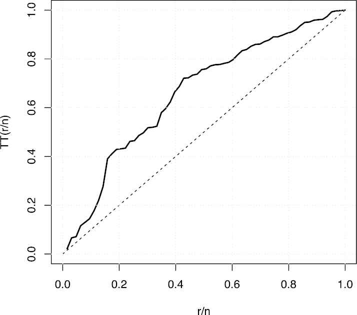
Graphical measure: The total time test TTT plot due to Aarset [3] is an important graphical approach to verify whether the data can be applied to a specific distribution or not. According to Aarset [3], the empirical version of the TTT plot is given by plotting Tr∕n=[∑i=1ryi:n+n−ryr:n]∕∑i=1nyi:n against r∕n, where r=1,…,n and yi:ni=1,…,n are the order statistics of the sample. Aarset [3] showed that the hazard function is constant if the TTT plot is graphically presented as a straight diagonal, the hazard function is increasing (or decreasing) if the TTT plot is concave (or convex). The hazard function is U-shaped if the TTT plot is convex and then concave, if not, the hazard function is unimodal. The TTT plots for data set is presented in Figure 6. These plots indicate that the empirical hazard rate functions of the data set is increasing. Therefore, the OHCEL distribution is appropriate to fit this data set.
Figure 6
Scaled-plot of the data set.
Here we obtain point and 95% confidence interval (CI) estimation of parameters of the OHCEL distribution by parametric bootstrap method for the real data set. We provide results of bootstrap estimation based on 1000 bootstrap replicates in Table 4. It is interesting to look at the joint distribution of the bootstrapped values in a scatter plot in order to understand the potential structural correlation between parameters.
Parametric Bootstrap
Non-parametric Bootstrap
Point Estimation
CI
Point Estimation
CI
a
2.096
(0.505, 4.949)
2.028
(0.517, 3.362)
λ
5.952
(3.063, 8.836)
5.888
(0.712, 34.743)
β
0.256
(0.054, 1.642)
0.290
(0.108, 0.661)
CI, confidence interval.
Table 4
Bootstrap point and interval estimation of the parameters a, λ and β.
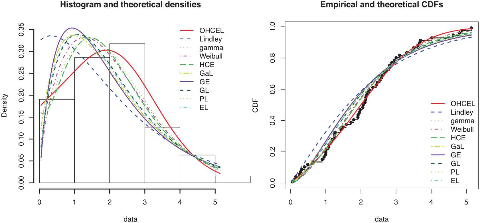
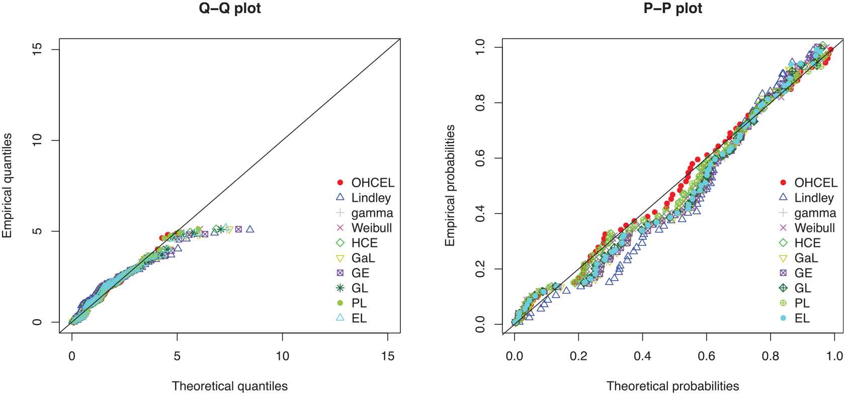
In the next, we fit the OHCEL distribution to the one data set and compare it with the HCE, Lidley, Generalized Lindley GL, Gamma Lindley GaL, Power Lindley PL, Exponential Lindley EL, gamma, generalized exponential (GE) and Weibull densities. Table 5 shows the MLEs of parameters, log-likelihood, Akaike information criterion AIC, Cramrvon Mises (W∗), Bayesian information criterion (BIC), Kolmogorov-Smirnov (K.S), AndersonDarling (A∗) and p−valueP statistics for the data set. The OHCEL distribution provides the best fit for the data set as it shows the lowest AIC, A∗ and W∗ than other considered models. The relative histograms, fitted OHCEL, HCE, Lindley, GL, GaL, PL, EL, gamma, GE and Weibull PDFs and the plots of empirical and fitted survival functions for data are plotted in Figure 7. The P−P plots and Q−Q plots for the OHCEL and other fitted distributions are displayed in Figure 8. These plots also support the results in Table 5. We compare the OHCEL model with a set of competitive models, namely:
Hyperbolic Cosine-Exponential distribution HCE [7]. The two-parameter HCE density function is given by
fx;a,λ=2aeae2a−1λe−λxcosha1−e−λx;x>0.
where a>0 and λ>0.
Lindley distribution [10]. The one-parameter Lindley density function is given by
fx;β=β21+β1+xe−βx;x>0,
where β>0.
GL distribution [16]. The three-parameter GL density function is given by
fx;θ,α,β=θα+1θ+βΓα+1xα−1α+βxe−θx;x>0,
where θ>0,α>0 and β>0.
Exponentiated EL distribution [12]. The two-parameter EL density function is given by
fx;θ,α=αθ21+θ1+xe−θx1−1+θx1+θe−θxα−1;x>0,
where θ>0 and α>0.
PL distribution [13]. The two-parameter PL density function is given by
fx;θ,α=αθ2θ+11+xαxα−1e−θxα;x>0.
where α>0 and θ>0.
GaL distribution [15]. The two-parameter GaL density function is given by
fx;θ,α=θ2α1+θ[α+αθ−θx+1]e−θx;x>0,
where θ>0 and α>0.
The two-parameter Weibull distribution is given by
fx;α,β=αβxβα−1e−xβα;x>0,
where α>0 and β>0.
The two-parameter Gamma distribution is given by
fx;α,θ=1θαΓαxα−1e−x∕θ;x>0
where α>0 and θ>0 and Γα=∫0∞tα−1e−tdt.
The two-parameter GE distribution is given by
fx;α,λ=αλe−λx1−e−λxα−1;x>0,
where α>0 and λ>0.
Model
MLEs of Parameters (s.e)
Log-likelihood
AIC
BIC
A∗
W∗
K.S
P
OHCEL
â=2.080.90
−98.02
202.04
208.47
0.22
0.02
0.06
0.95
λ̂=5.9414.99
β̂=0.260.33
HCE
â=3.690.67
−99.81
203.63
207.92
0.45
0.07
0.10
0.51
λ̂=0.890.09
Lindley
β̂=0.750.07
−104.57
211.15
213.29
2.13
0.41
0.15
0.08
GL
θ̂=1.040.17
−101.60
209.20
215.63
0.92
0.16
0.12
0.22
α̂=1.430.44
β̂=3.203.85
PL
θ̂=0.540.08
−99.58
203.17
207.45
0.49
0.06
0.09
0.56
α̂=1.380.12
EL
θ̂=0.920.10
−101.88
207.77
212.06
0.96
0.16
0.12
0.21
α̂=1.550.28
GaL
θ̂=0.900.09
−102.10
208.20
212.48
1.10
0.21
0.13
0.16
α̂=4.594.85
Weibull
α̂=1.620.16
−100.31
204.63
208.92
0.64
0.09
0.10
0.41
β̂=2.300.18
Gamma
α̂=1.90.31
−102.83
209.66
213.95
1.16
0.2
0.58
0.84
θ̂=0.910.17
GE
α̂=1.890.34
−103.54
211.09
215.37
1.31
0.23
0.14
0.13
λ̂=0.690.09
AIC, Akaike information criterion; EL, Exponential Lindley; GE, generalized exponential; GL, Generalized Lindley; GaL, Gamma Lindley; BIC, Bayesian information criterion; K.S, Kolmogorov-Smirnov.
Table 5
Parameter estimates (standard errors), log-likelihood values and goodness of fit measures.
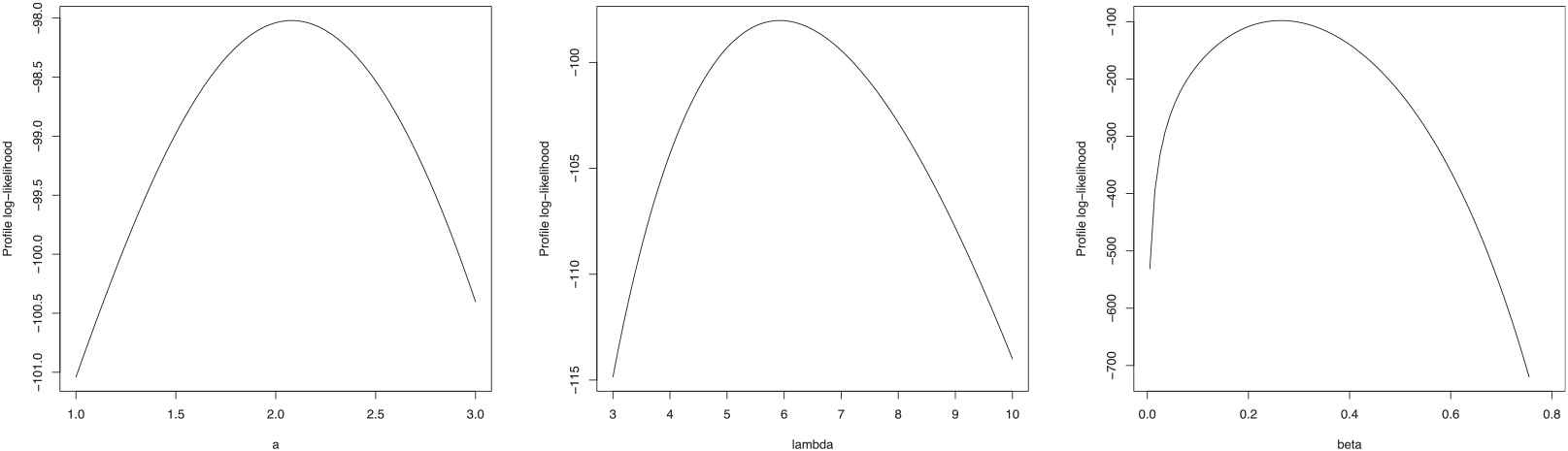
Figure 7
Profile-likelihood plots of distribution.
Figure 8
Estimated densities and Empirical and Estimated cdf for the data set.
Figure 9
Q-Q and P-P plots for the data set.
As mentioned in inference section, there are not closed expression for MLE estimation of parameters a, λ and β. We use numerical methods to obtain MLE estimation of these parameters. To evaluate the results of MLE estimation, We provide profile-likelihood plots of OHCEL distribution for each parameter in Figure 7.
7. CONCLUSION
In this article, a new model for the lifetime distributions is introduced and its main properties are discussed. A special submodel of this family is taken up by considering exponential distributions in place of the parent distribution F and Lindley distribution instead of the parent distribution G. We also show that the proposed distribution has variability of hazard rate shapes such as increasing, decreasing and upside-down bathtub shapes. Numerical results of maximum likelihood and bootstrap procedures for a set of real data are presented in separate tables. From a practical point of view, we show that the proposed distribution is more flexible than some common statistical distributions.
TY  - JOUR
AU  - Omid Kharazmi
AU  - Ali Saadatinik
AU  - Morad Alizadeh
AU  - G. G. Hamedani
PY  - 2019
DA  - 2019/11/25
TI  - Odd Hyperbolic Cosine-FG Family of Lifetime Distributions
JO  - Journal of Statistical Theory and Applications
SP  - 387
EP  - 401
VL  - 18
IS  - 4
SN  - 2214-1766
UR  - https://doi.org/10.2991/jsta.d.191112.003
DO  - 10.2991/jsta.d.191112.003
ID  - Kharazmi2019
ER  -