Journal of Statistical Theory and Applications

Volume 18, Issue 4, December 2019, Pages 375 - 386

Bayesian Analysis of Inverse Gaussian Stochastic Conditional Duration Model

Authors
C.G. Sri Ranganath*, N. Balakrishna
Department of Statistics, Cochin University of Science and Technology, Cochin, Kerala, 682022, India
*Corresponding author. Email: cg.srirang@gmail.com
Corresponding Author
C.G. Sri Ranganath
Received 20 September 2017, Accepted 21 October 2019, Available Online 20 November 2019.
DOI
10.2991/jsta.d.191031.001How to use a DOI?
Keywords
Stochastic conditional duration; Bayesian analysis; Markov Chain Monte Carlo; Inverse Gaussian distribution; Slice sampler
Abstract

This paper discusses Bayesian analysis of stochastic conditional duration model when the innovations follow inverse Gaussian distribution. Estimation is carried out by the methods of Markov Chain Monte Carlo. Applications of the model and methods are illustrated through simulation and data analysis.

Copyright
© 2019 The Authors. Published by Atlantis Press SARL.
Open Access
This is an open access article distributed under the CC BY-NC 4.0 license (http://creativecommons.org/licenses/by-nc/4.0/).

1. INTRODUCTION

The empirical analysis of durations between the occurrences of certain financial events is important in understanding the market behavior. To describe the evolution of such durations, Bauwens and Veredas [1] proposed a class of models called the stochastic conditional duration (SCD) models. One can refer Engle and Russell [2], Pacurar [3] for details on such duration models. The SCD model assumes that the conditional mean of durations between events is generated by a latent stochastic process. The likelihood based inference for such models requires evaluation of multiple integral with respect to latent variables. In view of these difficulties Bauwens and Veredas [1] estimated the parameters by quasi-maximum likelihood (ML) by expressing the model into a linear state space form and then applying Kalman filter method. Feng, Jiang and Song [4] proposed an extension to Bauwens and Veredas's [1] SCD model in order to capture the asymmetric behavior or leverage effect in the duration process. They adopted the Markov Chain Maximum Likelihood (MCML) approach proposed by Durbin and Koopman [5]. Strickland, Forbes and Martin [6] proposed a Bayesian Markov Chain Monte Carlo (MCMC) method in which the sampling scheme employed is a hybrid of the Gibbs and Metropolis-Hastings (MH) algorithm, with the latent vector sampled in blocks. Knight and Ning [7] discussed the empirical characteristic function (ECF) and the generalized method of moments estimation. Bauwens and Galli [8] developed a ML estimation based on the efficient importance sampling (EIS) method to estimate the parameters. Xu, Knight and Wirjanto [9] extended the SCD model of Bauwens and Veredas [1] by imposing mixtures of bivariate normal distributions on the innovations of the observation and latent equations of the duration process. Men, Kolkiewicz and Wirjanto [10] introduced a correlation between the error process and the innovations of the duration process and adopted Monte Carlo methods for estimation. Ramanathan, Mishra and Abraham [11] introduced a new procedure for estimation, filtering and smoothing in SCD models, based on estimating functions. Majority of the literature on SCD models assume that the errors follow either a Weibull, Gamma or exponential distribution. Balakrishna and Rahul [12] proposed a SCD model having inverse Gaussian (IG) distribution for innovations. In the present paper, we consider the Bayesian analysis of SCD model with IG error random variables. We propose Bayesian MCMC methods to estimate the parameters of the model. Here we follow the algorithm mentioned in Men, Kolkiewicz and Wirjanto [13], Edwards and Sokal [14] and Neal [15]. Since it is difficult to obtain the analytical conditional densities of observed data, the auxiliary particle filter (APF) in Pitt and Shephard [16] is employed to evaluate the likelihood function.

A brief review of IG SCD model is given in Section 2. The Bayesian estimation methodology and MCMC algorithm are discussed in Section 3. Simulation studies are carried out in Section 4. Section 5 presents the application of proposed method to real life data sets.

2. THE SCD MODEL

Let τi be the time of occurrence of an event (or transaction) of interest with τ0=0 and let Xi=τiτi1, i=1,2,,n be the ith trade duration, which is defined as the waiting time between two consecutive transactions of an underlying asset from time i1 to i.

The SCD model is defined by

Xi=eψiϵiψi=ϕψi1+ηi,i=1,2,,nψ0N(0,σ21ϕ2),
where |ϕ|<1 to ensure the stationarity of the process. Further, ηi follows independent and identically distributed (iid) N(0,σ2), so that {ψi} follows a Gaussian AR(1) sequence and {ϵi} is an iid sequence on the positive support with common pdf f(ϵi) and ηj is independent of ϵi i,j. Note that the model depends on the unobservable ψi, called the latent variable. Most of the SCD models available in the literature assume that the innovations follow iid exponential, gamma or Weibull distributions. One can refer Bauwens and Veredas [1], Strickland, Forbes and Martin [6], Knight and Ning [7], Durbin and Koopman [5] and so on for the details on such models. Xu, Knight and Wirjanto [9] proposed a SCD model by assuming a bivariate mixture of normal distribution for (ϵi,ηi). Balakrishna and Rahul [12] assumed an IG distribution for ϵi and estimated the model parameters by EIS method. In this paper we propose a Bayesian method for this SCD model with IG innovations. We consider the unit mean IG distribution for ϵi in the model (1).

A random variable X is said to have an IG distribution with parameters μ and λ, and is denoted by IG(μ,λ) if its probability density function (pdf) is of the form

f(x;μ,λ)=λ2πx3exp(λ(xμ)22μ2x),x>0,μ>0,λ>0.

If we restrict ϵi to follow a unit mean IG distribution then its pdf is of the form

fϵ(ϵi)=λ2πϵi3exp(λ(ϵi1)22ϵi),ϵi>0.

In order to develop an estimation procedure for the model let X=(x1,x2,x3,,xn1,xn) be a vector of observations from the model Eq. (1) and ψ=(ψ1,ψ2,,ψn) be a vector of associated latent variables, where denotes the transpose of a vector. If we denote the joint density function of (X,ψ) by f(X,ψ|θ), then the likelihood function of the parameter θ=(ϕ,σ,λ) based on the observations is

L(θ;X)=f(X,ψ|θ)dψ,
which is an n-fold integral with respect to ψ. We need to evaluate this integral to obtain the likelihood function. Toward that end some numerical methods such as MCMC are to be used. In the next section, we propose a Bayesian method for estimating the parameters.

3. BAYESIAN ESTIMATION

We consider the problem of estimation for the SCD model when the innovations of the durations follow an IG distribution in a Bayesian framework. By Bayes theorem, the joint conditional distribution of ψ and θ given the observations is

f(θ,ψ|X)f(X|ψ,θ)f(ψ|θ)f(θ),
where f(X|ψ,θ) is the density of X given (θ,ψ), f(ψ|θ) is the density of ψ and f(θ) is the prior density of θ. Bayesian inference on (θ,ψ) is based upon the posterior distribution f(θ,ψ|X). From this joint posterior, the marginal f(θ|X) can be used to make inferences about the parameters of SCD model with IG innovations and the marginal f(ψ|X) provides the inference about the latent variables. We assume that the prior distributions of ϕ,σ,λ are mutually independent. We take prior distribution of ϕ as a normal truncated in the interval (1,1) which results in flat density over the supporting region. For σ2 we take an inverse gamma prior distribution as in Pitt and Shephard [16], which is a conjugate prior. For the parameter λ, we use a truncated Cauchy prior distribution with density
f(λ)11+λ2,λ>0,
which was also considered by Bauwens and Lubrano [17].

To construct an appropriate Markov Chain sampler, the joint posterior should be expressed as proportional to various conditional distributions. So in Eq. (5), the joint posterior, f(ψ|θ) is further decomposed into a set of conditionals f(ψi|ψi,θ,X), where ψi means all terms of ψ except ψi. Here, since ψ is a vector of latent variables, it is difficult to sample from these univariate conditional distributions. So we follow the MCMC algorithm proposed by Men, Kolkiewicz and Wirjanto [13] for estimation.

While developing MCMC algorithm, the latent variables are augmented with the vector of parameters and then the estimation is carried out. We start drawing samples from the conditional posterior distribution of the latent variable ψ and the parameters θ. The sampling algorithm required to draw the samples from each conditional posterior and the associated steps are detailed below.

The parameters θ=(ϕ,σ,λ) are initialized with values (0.5,0.5,1) and then the initial value of ψ is generated from latent AR(1) model by using these values of θ.

Step 1. Sample ψ=(ψ1,ψ2,,ψn) by drawing ψi from f(ψi|ψi,X,θ) for i=1,2,3,,n. By employing the markovian structure of the model in (1), f(ψi|ψi,X,θ) can be expressed as f(ψi|ψi1,ψi+1,X,θ). A single-move MH algorithm is used to sample ψi. The conditional distribution of latent random variables ψi, given the other parameters in the model have been previously obtained is given by

f(ψ1|X,ψ2,θ)f(x1|ψ1)f(ψ1|θ)f(ψ2|ψ1,x1,θ),
f(ψi|X,ψi1,ψi+1,θ)f(xi|ψi)f(ψi|ψi1,xi1,θ)f(ψi+1|ψi,xi,θ)i=2,,n1,
f(ψn|X,ψn1,θ)f(xn|ψn)f(ψn|ψn1,xn1,θ),
where f(xi|ψi), i=1,2,,n are the conditional density functions of the durations, f(ψ1|θ) is the density of the latent state ψ1, f(ψi|ψi1,xi1,θ) is the conditional density of ψi given ψi1 and f(ψi+1|ψi,xi,θ) is the conditional density of ψi+1 given ψi. Since xn is the last observation, the posterior distribution of ψn depends only on xn, xn1 and ψn1. The conditional distribution of ψ1 and ψn are given in Appendix A. If the conditional distribution does not possess a simple form as in the present case then it is not possible to draw the samples directly. In such cases one of the options is to consider an accept/reject method. Following Men, Kolkiewicz and Wirjanto [13] we use a single-move Metropolis Hastings algorithm to sample the latent states, where the proposal distribution is simulated by slice sampler method. The slice sampler method proposed by Edwards and Sokal [14] and Neal [15] is a method to sample random variables which do not have simple pdfs or their pdfs are known up to a normalizing constant. As the slice sampler adapts to the analytical structure of the underlying density, it is more efficient. Also it ensures faster convergence to the underlying distribution. So, to generate random variates from the conditional distribution we employ the method of slice sampler. While analyzing a data, we estimate these unobservable latent variables ψ, usingAPF method proposed by Pitt and Shephard [16]. In the following discussion, we obtain specific forms of the required samplers.

For i=2,3,,n1,

(ψi|ψi1)N(ϕψi1,σ2) and (ψi+1|ψi)N(ϕψi,σ2).

Substituting for the corresponding normal densities and on simplifying the square terms we get

f(ψi|ψi,θ)exp((1+ϕ2)2σ2(ψi22ψi(ϕϕ2+1(ψi1+ψi+1))))N(ω1,σ12),
where ω1=ϕ1+ϕ2ψi1+ψi+1 and σ12=σ21+ϕ2.

Hence the conditional posterior distribution of ψi can be represented as

f(ψi|X,ψi1,ψi+1,θ)f(xi|ψi)f(ψi|ψi1,θ)f(ψi+1|ψi,θ)
λeψixi3expλ(xieψi)22eψixiexp(ψiϕψi1)22σ2exp(ψi+1ϕψi)22σ2(λexp(ψ))12expλ(xieψi)22eψixiexp(ψiai)22b,
where ai=ϕ(ψi+ψi+1)1+ϕ2 and b=σ21+ϕ2.

The posterior distribution in (8) is proportional to a product of three positive functions and data cannot be simulated directly from them. So we propose a method of slice sampler whose algorithm is given below.

Slice sampler algorithm for ψi. Let us rewrite the conditional distribution in (8) as

g(ψi)expλ(xieψi)22eψixiexp(ψia1i)22b,
where a1i=ai+b2 and follow the algorithm given below.

To start the slice sampling procedure, the sampled value of ψi from the last MCMC step is set as the initial value.

  1. Initialize ψi(0). Set t = 0.

  2. Draw a random observation u1 uniformly from the interval 0,expλ(xieψi(t))22eψi(t)xi. Then we define an interval for ψi through the inequality u1expλ(xieψi)22eψixi, which is equivalent to

    ψilogxi(1+1ϵi2)21(log(u1))λ.

  3. Similarly draw a random observation u2 uniformly from the interval 0,exp(ψia1i(t))22b, where a1i(t) is calculated from Eq. (9). We define an interval for ψi through the inequality u2exp(ψia1i)22b, which is equivalent to

    a1i(t)2blog(u2)ψia1i(t)+2blog(u2).

  4. Draw ψi(t+1) uniformly from the interval maxlogxi(1+1ϵi2)21(log(u1))λ,a1i(t)2blog(u2),a1i(t)+2blog(u2) determined by the inequalities (10) and (11).

  5. Stop, if a stopping criterion is met; otherwise, set t=t+1 and repeat from ii.

Step 2. Sample ϕ. The prior distribution of ϕ is assumed to follow a univariate normal distribution truncated in the interval (-1,1). Given a truncated normal prior distribution, ϕN(αϕ,βϕ2) and the other parameters in the model have been previously sampled, the conditional distribution of ϕ is

f(ϕ|X,σ2,λ)f(ψ|θ,X)f(ϕ).=f(ψ1|θ,X)i=2nf(ψi|ψi1,xi,θ)exp(ϕαϕ)22βϕ2.Ndc,1c1ϕ2,
where c=i=2nψi2σ2+1βϕ2, d=i=2nψiψi1σ2+αϕβϕ2. The conditional distribution of ϕ is given in Appendix A. It is proportional to the product of a normal distribution and a positive function. Hence we can use the slice sampling method to sample the parameter ϕ.

Step 3. Sample σ2. We sample σ2 by taking an inverse gamma prior distribution, i.e., σ2 inverse Gamma (ασ2,βσ2), where ασ2 and βσ2 are hyperparameters. As the prior for σ2 is a conjugate prior the sampling is carried out by simulating from the inverse Gamma distribution with the corresponding parameters obtained. The conditional distribution of σ2 is presented in Appendix A.

Step 4. Sample λ. The conditional distribution of λ is

f(λ|X,ψ,ϕ,σ2)=f(X|ψ,λ)f(λ).=f(λ)i=1nλeψixi3expλ(xieψi)22eψixi,
where f(λ) is a prior density of λ, given by (6). Here the samples cannot be simulated directly from (13). So we use a random walk MH algorithm with standard normal distribution as the proposal distribution to sample λ. The acceptance probability is computed using (13).

The following is a summary of the procedure used to sample (θ,ψ).

  • Sample ψ using the single-move MH algorithm with proposal distribution simulated by the method of slice sampling which is briefly explained in Step 1.

  • Sample ϕ from (12) following the explanations in Step 2.

  • Sample σ2 directly from the inverse Gamma density using Step 3.

  • Sample λ using a random walk MH algorithm with the acceptance probability computed through (13) given in Step 4.

In the next section we demonstrate the applications of the above methods through a simulation study.

4. SIMULATION STUDY

A simulation study is carried out to assess the performance of the Bayes estimators, described in the previous section. We generate 5000 observations from the model (1). Then the MCMC algorithm discussed in Section 3 is run and first 25000 iterations were discarded as burn-in from 100000 iterations. The parameters are estimated and the simulation results are tabulated in Table 1. The plots of histograms of posterior samples of ϕ, σ2, λ are shown in Figure 1 (a), 1 (b) and 1 (c) respectively. The trace plots are shown in Figure 2 (a), 2 (b) and 2 (c) respectively.

ϕ σ λ
True. 0.75 1.5 1
Est. 0.763302 1.529561 0.999191
mse. 0.000039 0.000094 0.0000039
HPD CI(95%) (0.74633, 0.78840) (1.47808, 1.57561) (0.9557, 1.1477)

True. 0.85 1.5 1
Est. 0.84699 1.55057 0.999242
mse. 0.0000322 0.000095 0.0000041
HPD CI(95%) (0.82633, 0.86840) (1.49808, 1.58561) (0.9657, 1.1413)

Highest probability density Confidence interval (HPD CI)
Table 1

True and estimated parameters of the IG-SCD model.

Figure 1

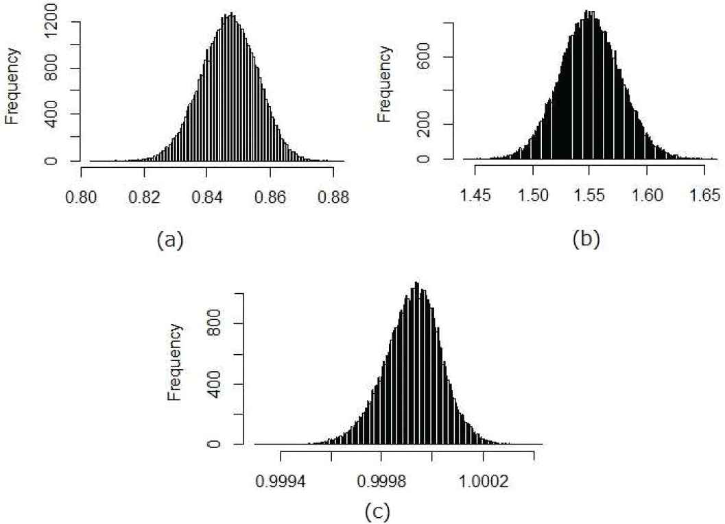
Histogram of the posterior samples using simulated data.

Figure 2

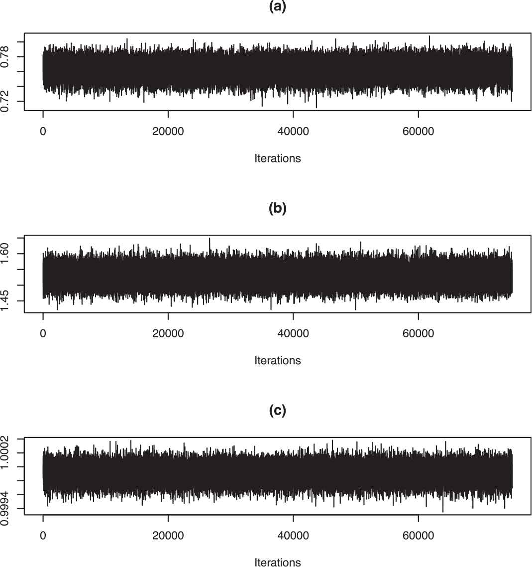
Trace plots of the posterior samples using simulated data.

To illustrate the application of Bayesian estimation method we analyze two sets of data. We perform model diagnosis based on the residuals to explain model adequacy. The residuals of SCD model with IG innovations are defined as ϵî=xieψî, where ψî is the estimator of ψi. The estimators of the parameters ϕ, σ and λ can be obtained by the MCMC algorithm discussed in Section 3. To obtain the estimates of the unobservable component ψi, we employ an APF proposed by Pitt and Shephard [16]. This method is described in the following subsection:

4.1. Particle Filter

Particle filters are a class of simulation-based filters that recursively approximate the filtering distribution using a collection of particles with some probability masses. The particles are samples of unknown states from the state space, and the particle weights are probability mass computed by Bayes theory. The basic idea is the recursive computation of relevant probability distribution and approximation of probability distribution.

By successive conditional decomposition, the likelihood of the IG-SCD model is

f(X|θ)=f(x1|θ)i=2nf(xi|i1,θ),
where i=σ(x1,x2,,xi), the sigma field generated by (x1,x2,,xi) is the information known at time i. The conditional density of xi+1 given θ and i is given by
f(xi+1|i,θ)=f(xi+1|ψi+1,θ)dF(ψi+1|i,θ)=f(xi+1|ψi+1,θ)f(ψi+1|ψi,θ)dF(ψi|i,θ).

The difficulty in obtaining an analytical form of the above integral leads to the utilization of APF. Suppose that we have a particle sample {ψi(t),t=1,2,,N} of ψi from the filtered distribution (ψi|i,θ) with weights { πt,t=1,2,,N} such that t=1Nπt=1. From this sample, the one-step ahead predictive density of ψi+1 is

f(ψi+1|Fi,θ)t=1Nπtf(ψi+1|ψi(t),θ)

The one step ahead prediction distribution of ψi+1 can then be sampled and the conditional density (15) can be evaluated numerically by

f(xi+1|Fi,θ)t=1Nπtf(xi+1|ψi+1(t),θ),
where ψi+1(t) are particles from the prediction distribution of (ψi+1|i,θ). The predictive density of ψi+1 should be known for the approximation (16) to be feasible. From latent AR(1) process, we have ψi+1 has a conditional normal distribution ψi+1N(ϕψi,σ2).

Given the particle sample from a filtered distribution (ψi|i,θ) we need to sample (ψi+1|i+1,θ). For that, we follow the procedure of Chib, Nardari and Shephard [18] and Men, Kolkiewicz and Wirjanto [13], which is summarized below.

4.1.1. Algorithm for APF

  1. (a) Given a sample { ψi(t),t=1,2,,N} from (ψi|i,θ), calculate the expectation ψ̂i+1(t)=E(ψi+1|ψi(t)) and

    πt=f(xi+1|ψ̂i+1(t),θ),t=1,2,,N
    and sample N times with replacement the integers 1,2,…,N with probability πt̂=πtt=1Nπt. Let the sampled indexes be k1,k2,,kN and associate these with particles { ψ̂i(k1),ψ̂i(k2),,ψ̂i(kN)}.

  2. For each value of kt from 1(a), sample the values {ψi+1(1),,ψi+1(N)} from

    ψi+1(t)=ϕψi(kt)+ηi+1,t=1,,N
    where ηi+1N(0,1).

  3. Calculate the weights of the values {ψi+1(1),,ψi+1(N)} as

    πt=f(xi+1|ψi+1(t),θ)f(xi+1|ψ̂i+1(kt),θ),t=1,2,,N
    and using these weights resample the values {ψi+1(1),,ψi+1(N)} N times with replacement to obtain a sample {ψi+1(1),,ψi+1(N)} from the filtered distribution (ψi+1|i+1,θ). Here we use N=2000.

5. DATA ANALYSIS

We demonstrate the applications of the model, by analysing two sets of data. Data sets are on intraday trades of IBM OHLC bar data downloaded from Algoseek Website and intraday trades of US Brent Crude Oil downloaded from the Website of a Swiss Forex bank. Only trades between 9:30:00 am and 4:00:00 pm are recorded as this is the normal trading hour.

5.1. IBM Trades Data

The model is applied to intraday IBM trades data as on 16th June 2015. Consider the 1 second Trade OHLC Bar data with a sample size of 6708 observations. The trade durations are defined as the time intervals between consecutive trades, measured in seconds. We ignore the zero trade duration and the time plot of the nonzero intraday IBM trade duration series is shown in Figure 3. Now, removing the effect of the diurnal pattern we take the adjusted time duration (Tsay [19], pp. 298–300) to model the intraday pattern. In Table 2 the summary statistics of IBM trades data are given.

Figure 3

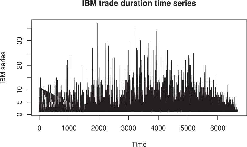
IBM trade duration time series.

Statistic IBM Trades Data
Sample size 6708
Minimum 1
Maximum 37
Mean 3.48
Median 2
Table 2

Descriptive statistics for IBM trades data.

The estimation of the parameters is carried out by the MCMC algorithm described in Section 3 and the estimates are provided in Table 3. For model diagnosis we compute residuals, ϵî= xieψî, where ψî is the estimator of ψi which is obtained by APF. If the fitted model is adequate then the Autocorrelation function (acf) of {ϵî} will be negligible. The residual acf plot given in Figure 4 indicates that they are uncorrelated. Bauwens and Veredas [1] considered the time series version of Spearman's ρ correlation coefficient and the p-value plots instead of the Ljung-Box statistic. Here we follow a rank portmanteau statistic given in Dufour and Roy [20] to check the lack of autocorrelation of the obtained residuals. The p-value obtained is 0.7. Also the run test confirms the independence of the residuals {ϵî}. In Figure 5 the histogram of the residuals is superimposed by the IG density curve for the IG-SCD model. So it can be concluded that the fitted model is adequate for explaining the dynamics, which generated the data.

ϕ σ λ
Est. 0.69803 1.2366 1.1566
Std error 0.00143 0.00906 0.00658
Table 3

Estimated parameters of the IG-SCD model based on IBM Trades duration data.

Figure 4

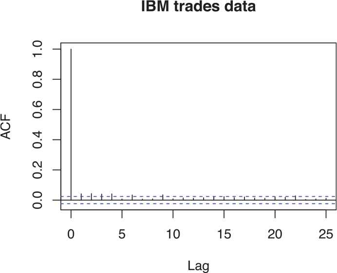
ACF plot of residuals.

Figure 5

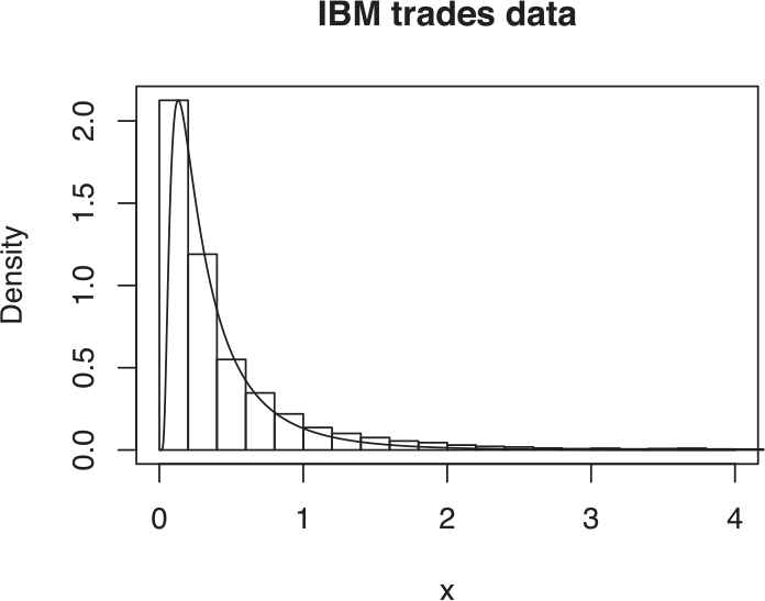
Histogram of residuals superimposed by inverse Gaussian density for IG-SCD model.

5.2. US Brent Crude Oil

The second set of data is the intraday trades data of US Brent Crude Oil downloaded from the Website of a Swiss Forex bank and Marketplace. The intraday trade of the Brent Crude Oil on 20 February 2017 is considered. Taking the normal trading hours and ignoring the zero durations the sample size obtained is 1625 trade durations. The time plot of the nonzero intraday durations and the time plot of the adjusted duration series is shown in Figures 6 and 7. The summary of data is given in Table 4.

Figure 6

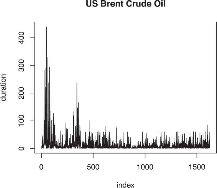
Duration plot of US brent crude oil.

Figure 7

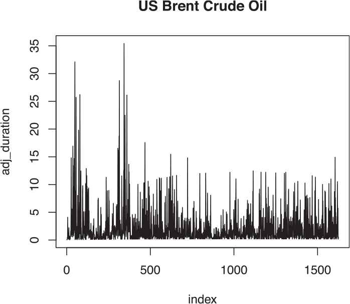
Adjusted duration plot of US brent crude oil.

Statistic IBM Trades Data
Sample size 1625
Minimum 1
Maximum 439
Mean 14.4
Median 6
Table 4

Descriptive statistics for US Brent Crude Oil Trades data.

The parameters are estimated by the algorithm mentioned in Section 3 and are tabulated in Table 5. From the residual plot given in Figure 8 and the p-value (= 0.8) obtained from rank portmanteau statistic we conclude that the residuals are independent. The superimposition of the histogram of the residuals and the IG density curve in Figure 9, shows a good fit of error distribution.

ϕ σ λ
Est. 0.77263 1.34885 0.945069
std error. 0.00567 0.00975 0.01018
Table 5

Estimated parameters of the IG-SCD model based on US Brent Crude Oil trades duration data.

Figure 8

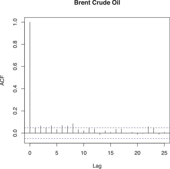
Residual plot of US brent crude oil.

Figure 9

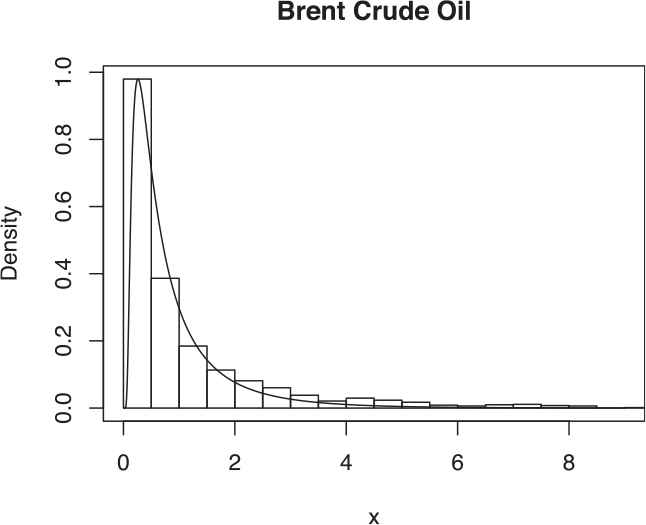
Histogram of residuals superimposed by inverse Gaussian density for inverse Gaussian-stochastic conditional duration (IG-SCD) model.

6. CONCLUSION

In this article we considered the Bayesian estimation of SCD model with IG error random variables. The slice sampling within an MCMC estimation methodology and the APF method are utilized to estimate the parameters and the latent states of the model. Simulation study shows that the proposed estimation method is reliable. Two sets of financial data are considered to demonstrate the utility of the model. The non-parametric tests applied to residuals support the assumptions on the errors. However, more rigorous statistical tests are to be developed to perform model diagnosis in the presence of latent variables.

CONFLICT OF INTEREST

The authors declare no conflict of interest.

ACKNOWLEDGMENTS

The authors thank the editor and the reviewers for their careful reading of the article. Sri Ranganath acknowledge Kerala State Council for Science Technology & Environment, for the financial assistance for carrying out this research work. The research of N. Balakrishna is partially supported by the DST SERB under the project No. SR/S4/MS:837/13.

APPENDIX A

The conditional distribution of parameter ϕ is

f(ϕ|X,σ,λ)f(ψ|θ,X)f(ϕ)=f(ψ1|θ,X)i=2nf(ψi|ψi1,θ,X)exp(ϕαϕ)22βϕ2exp(1ϕ2)ψ122σ2exp(i=1n(ψiϕψi1)22σ2)exp(ϕαϕ)22βϕ2(1ϕ2)12exp12ϕ2i=1nψ12σ2+1βϕ22ϕi=1nψiψi1σ2+αϕβϕ2(1ϕ2)12Ndc,1c1ϕ2,
where c=i=1nψ12σ2+1βϕ2, d=i=2nψiψi1σ2+αϕβϕ2. The conditional distribution of parameter σ2, by taking an Inverse Gamma prior is
f(σ2|X,ϕ,λ)=f(ψ|θ,X)f(ασ2,βσ2)=f(ψ1|θ,X)i=2nf(ψi|ψi1,θ,X)f(ασ2,βσ2)expψi2(1ϕ2)2σ2×expi=2N(ψiϕψi1)22σ2×(σ2)n2×(βσ2)ασ2Γ(ασ2)(σ2)ασ21exp(βσ2σ2)(σ2)(2ασ2)n+22expψi2(1ϕ2)i=2N(ψiϕψi1)2+2βσ22σ2inverseGamma(a,b).
where a=ασ2+n2 and b=(1ϕ2)(ψi)22+12i=2n(ψiϕψi1)2+βσ2.

The conditional distribution of parameter ψ1 is

f(ψ1|X,ψ2,θ)f(x1|ψ1)f(ψ1|θ)f(ψ2|ψ1,x1,θ)=f(x1|ψ1)exp(1ϕ2)ψ122σ2exp(ψ2ϕψ1)22σ2.

The conditional distribution of parameter ψn is

f(ψn|X,ψn1,θ)f(xn|ψn)f(ψn|ψn1,xn1,θ)f(xn|ψn)exp(ψnϕψn1)22σ2.

REFERENCES

19.R.S. Tsay, An introduction to analysis of financial data with R, John Wiley & Sons, Hoboken, 2013. https://www.wiley.com/en-us/An+Introduction+to+Analysis+of+Financial+Data+with+R-p-9780470890813
Journal
Journal of Statistical Theory and Applications
Volume-Issue
18 - 4
Pages
375 - 386
Publication Date
2019/11/20
ISSN (Online)
2214-1766
ISSN (Print)
1538-7887
DOI
10.2991/jsta.d.191031.001How to use a DOI?
Copyright
© 2019 The Authors. Published by Atlantis Press SARL.
Open Access
This is an open access article distributed under the CC BY-NC 4.0 license (http://creativecommons.org/licenses/by-nc/4.0/).

Cite this article

TY  - JOUR
AU  - C.G. Sri Ranganath
AU  - N. Balakrishna
PY  - 2019
DA  - 2019/11/20
TI  - Bayesian Analysis of Inverse Gaussian Stochastic Conditional Duration Model
JO  - Journal of Statistical Theory and Applications
SP  - 375
EP  - 386
VL  - 18
IS  - 4
SN  - 2214-1766
UR  - https://doi.org/10.2991/jsta.d.191031.001
DO  - 10.2991/jsta.d.191031.001
ID  - SriRanganath2019
ER  -