
Network with Sub-networks: Layer-wise Detachable Neural Network
- DOI
- 10.2991/jrnal.k.201215.006How to use a DOI?
- Keywords
- Model compression; neural networks; multilayer perceptron; supervised learning
- Abstract
In this paper, we introduce a network with sub-networks: a neural network whose layers can be detached into sub-neural networks during the inference phase. To develop trainable parameters that can be inserted into both base-model and sub-models, first, the parameters of sub-models are duplicated in the base-model. Each model is separately forward-propagated, and all models are grouped into pairs. Gradients from selected pairs of networks are averaged and used to update both networks. With the Modified National Institute of Standards and Technology (MNIST) and Fashion-MNIST datasets, our base-model achieves identical test-accuracy to that of regularly trained models. However, the sub-models result in lower test-accuracy. Nevertheless, the sub-models serve as alternative approaches with fewer parameters than those of regular models.
- Copyright
- © 2020 The Authors. Published by Atlantis Press B.V.
- Open Access
- This is an open access article distributed under the CC BY-NC 4.0 license (http://creativecommons.org/licenses/by-nc/4.0/).
1. INTRODUCTION
Deep Neural Networks (DNNs) have gained attraction in recent years owing to their ability to provide state-of-the-art performance in various applications, including image recognition, object detection, and speech recognition. However, deploying DNNs on mobile devices is challenging because the mobile devices have diverse specifications. This raises the question of how to effectively design DNNs given mobile phone specifications. To address this question, two main aspects of DNNs can be optimized.
The first aspect is the performance of DNNs. In general, there is assumption that increasing the number of layers of a DNN leads to better the model performance. One widely used example is the trend observed in the number of layers in the ImageNet Large Scale Visual Recognition Competition (ILSVRC). AlexNet [1], the model that won ILSVRC-2012, consists of eight layers, while ResNet [2], the winner of ILSVRC-2015, contains 152 layers. Compared with AlexNet, ResNet reduces the top-5 test error rate from 15.3 to 3.57.
Although a larger number of layers may reduce the test-error rate of a model, this has a trade-off with the second aspect of DNNs: latency. A larger number of layers in a DNN signifies that there is a larger number of parameters to compute. This increases the memory footprint, which is crucial for a mobile device. A larger number of parameters also leads to an increase in the overall power consumption due to refreshing, moving, and computing data.
To solve this optimization problem, we can select a model that achieves real-time performance given a mobile device specification. However, if the user prefers performance over latency, this method does not satisfy the user demand. Another approach is to allow the user to select the preference and subsequently match this preference to the most suitable model. However, this method has a larger memory footprint due to storing various models on the mobile device. To satisfy user selectivity in both performance and latency without a large memory footprint, we propose a Network with Sub-networks (NSN), which is a DNN whose layers can be removed without significantly reducing in the performance.
Generally, if one layer of a DNN is detached during inference, the performance of the model is reduced. To explain our hypothesis, we compare a DNN to a feature extraction model. In the first layer, the model extracts low-level features, while in the last layers, it recombines the low-level features into high-level features. This process creates a dependency relationship between each layer.
In this study, we propose a training method that allows an NSN to dynamically adapt to the removal of weight layers. The two processes in this method are called copying learn-able parameters and sharing gradient, and both are designed to optimize the learn-able parameters for models, both with and without a layer to be detached.
2. RELATED WORK
In this section, we describe two related studies that are similar to our proposed method.
2.1. Slimmable Neural Network
Slimmable Neural Networks (SNNs) [3] greatly influenced this research. If our proposed method adds or removes weights in the depth-wise or layer-wise direction, SNNs append or detach weights in the width-wise direction. The discrete range of possible widths of networks must be predefined as the switch. The main research problem in this study is that mean and variance of activations produced from different-width layers are generally diverse. SNNs propose switchable batch normalization for each possible width to correct the mean and variance of SNNs.
2.2. BranchyNet
BranchyNet [4] is a neural network that can reduce the number of floating point operations during inference depending on the complexity of the input data. In BranchyNet, the output activations between immediate layers of neural networks, are connected with a branch, which consists of the layers and a classifier. If the prediction of input data of that branch classifier has higher confidence than a predefined threshold, then the output of the model is produced early from that branch. However, if the confidence is lower than the predefined threshold, then the features are passed to the deeper layers. BranchyNet can thus automatically detect complex data and determine whether to process these data further into the deeper layers or produce an early prediction through the branch.
3. NETWORK WITH SUB-NETWORKS
Network with sub-networks are designed to provide the layer-wise detachability for DNNs. Specifically, NSNs insert a smaller model into a larger model. Therefore, if the layers of the larger model are detached, the larger model becomes the smaller model. To implement this concept for DNNs, NSNs must have the same learning parameters for the smaller and larger models during both forward and backward propagation.
There are two types of models in NSNs: a base-model and sub-model. The base-model is defined as a DNN with n hidden layers, where n is a positive integer greater than zero. From the base-model, we can create n sub-models. Each sub-model is mapped with 0, …, n − 1 hidden layers. With this concept, the largest sub-model takes all of the layers of the base-model except the input layer. Furthermore, the second largest sub-model takes all of the layers of the largest sub-model except the input layer. This can be performed repeatedly until we obtain the sub-model with no hidden layers.
In the next section, we describe two processes in our purposed method: copying learn-able parameters and sharing gradient. These processes are designed to be applied repeatedly in every mini-batch training. In addition, they are designed to enforce the similarity of weight values between the base-model and sub-model during forward and backward propagation.
3.1. Copying Learn-able Parameters
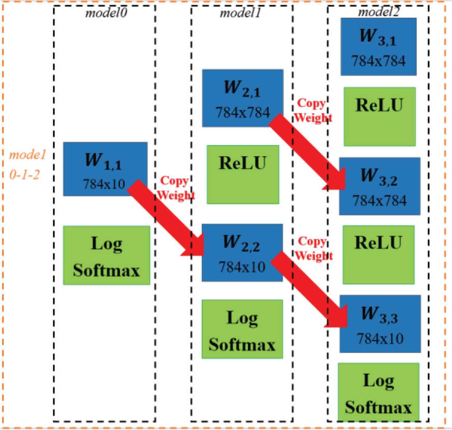
The goal of copying learn-able parameters is to insert the sub-model into the base-model. To ensure the similarity between the weight and bias parameters for each model, the weights and biases are copied from the smaller sub-model to the larger sub-model. This process is repeated up to the base-model, as express in Equation (1) and Figure 1. Here, Wo,m is a weight variable, o is an integer indicating the order of the layer, and m is an integer indicating the model number.
After applying this process, if we remove the input layer of the base-model with the non-linear activation function, the base model becomes the sub-model.
Sharing gradient in model0-1-2 section. The gradients are shared from the sub-model to the base-model, pair by pair. Only the input layer of W3,1 is regularly updated without sharing.
3.2. Sharing Gradient
Sharing gradient is designed to constraint the learnable-variables to able to be perform in two or more networks. First, all of the models are forward propagated. During back propagation, the gradients from each model are collected separately. Each model is paired from the sub-model without any hidden layer to the sub-model with a hidden layer. This process is repeated until the sub-model with n − 1 hidden layers is paired to the base-model. The gradients from each model’s pair are averaged, and the weights and bias are updated. The sharing gradient process is expressed in Equation (2) and Figure 2 where lr is the learning rate and L is the loss function.
The reason for using the sharing gradient process for only a pair of models is that when sharing more than a gradient pair, the optimization becomes too complex. In this case, the performance of the NSN does not reach the optimal point. Nonetheless, there is only an input layer of the base-model that does not have a pair. This input layer is updated with regular back propagation without sharing gradient.
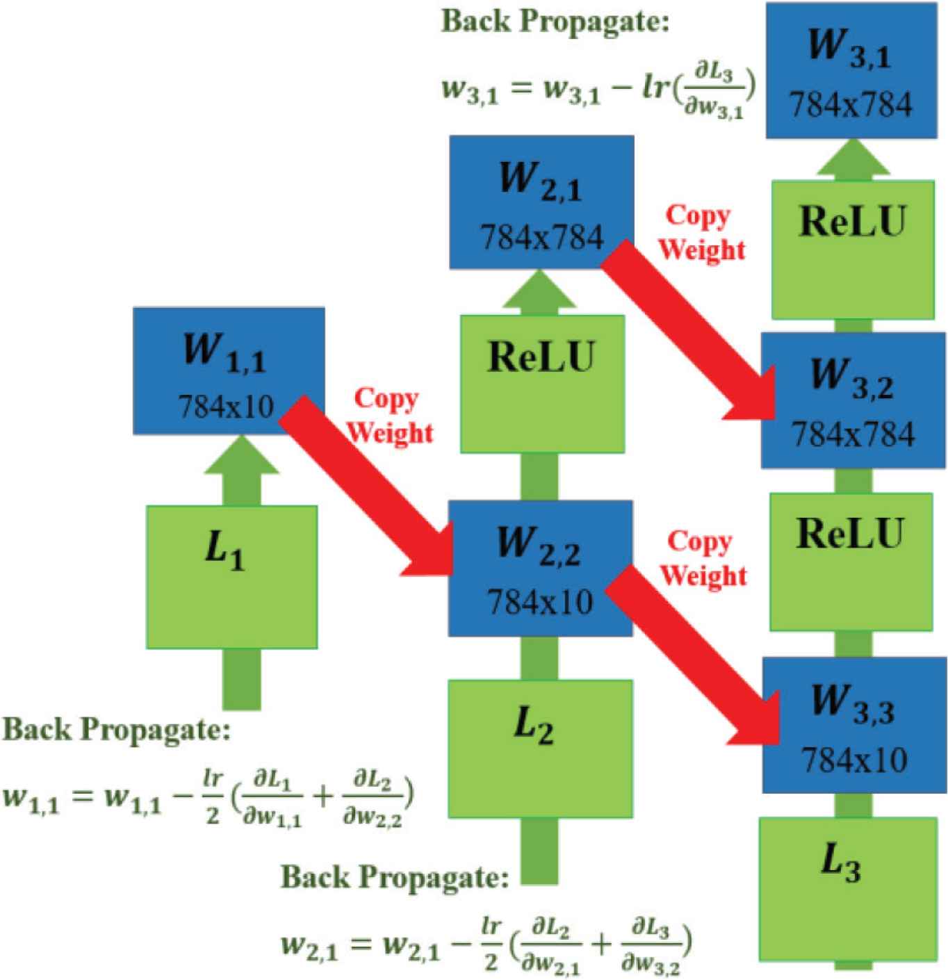
Illustration of a network with sub-networks and the copying learn-able parameters process. Here the base-model is a two hidden layer DNN and the sub-model is a one hidden layer DNN and a softmax-regression model. Lm is the loss function of the m models. In the figure, the weight, Wo,m follows with the size of the weight array. Copying learn-able parameters leads W1,1, W2,2 and W3,3 to have exactly the same weight.
4. EXPERIMENTS
Experiments were conducted using a hand-written digit image dataset, MNIST [5], and fashion product image dataset, Fashion-MNIST [6]. The MNIST and Fashion-MNIST datasets both consisted of 60,000 training images and 10,000 test images. Each image in both datasets was a 28 × 28 pixel grayscale image. Each image pixel was pre-processed into the range [0, 1] by dividing all pixel values by the maximum intensity pixel value, 255.
A Multi-layer Perceptron (MLP) was applied with rectified linear unit as the non-linear activation function. Only the last layer was applied with log-softmax with the cost function as cross-entropy loss. The input layer of the MLP was applied with a dropout [7] rate of p = 0.8. The hidden layers were applied with a dropout rate of p = 0.5. For softmax-regression, we did not apply dropout in the model, as it was already under-fitting. The models were further regulated using the L2-weight penalty.
We applied Stochastic Gradient Descent (SGD) with momentum [8] of α = 0.9. We applied with slightly different format of SGD with momentum comparing to standard framework. From Tensorflow [9], a neural networks framework, the format of SGD with momentum is defined in Equation (3), where V is the gradient accumulation term, t is the batch iteration step, and G is the gradient at t + 1. Our format of SGD with momentum is illustrated in Equation (4). After V is determined, both formats use Equation (5) to update the weight W.
Network with sub-networks performed better with our format of SGD with momentum than the regular format or TensorFlow format at α = 0.9. We speculate that NSNs required a higher proportion of the gradient accumulation V to converge than with the current gradient G. However, with regularly trained DNNs, our format of SGD with momentum performed slightly worse in term of test accuracy. To perform a fair comparison between both types of models, the regularly-trained models were trained with Equation (3), TensorFlow format SGD with momentum. Our proposed method models were trained with Equation (4), our format of SGD with momentum. We set the training batch to 128. Each model trained for 600 epochs. We reported the best test accuracy that occured during the training. The initial learning rate was lr = 0.3 and was stepped down by one third every 200 epochs.
The experiment consists of two sections. The first section is model0-1, or the base-model as an MLP with a hidden layer (model1) with a sub-model as the soft-max regression (model0). The second section is model0-1-2, or the base-model as a two hidden layers MLP (model2). The sub-models are an MLP with a hidden layer (model1), and the soft-max regression (model0). An illustration of model0-1-2 is presented in Figure 2. The baseline models, which are trained regularly, are referred to as ref-model followed by the number of hidden layers. For example, ref-model1 is the baseline MLP with one hidden layer. The MNIST results of the baseline models are presented in Table 1, while the Fashion-MNIST results of the baseline model are presented in Table 2.
| Test accuracy | Number of parameters | Regularization parameter | |
|---|---|---|---|
| ref-model2 | 0.9886 | 1.24 M | 1 × 10⁻⁵ |
| ref-model1 | 0.9882 | 0.62 M | 5 × 10⁻⁶ |
| ref-model0 | 0.9241 | 7.85 K | 9 × 10⁻⁵ |
Results of MNIST classification of base-line models
| Test accuracy | Number of parameters | Regularization parameter | |
|---|---|---|---|
| ref-model2 | 0.9089 | 1.24 M | 1 × 10⁻⁵ |
| ref-model1 | 0.9085 | 0.62 M | 5 × 10⁻⁶ |
| ref-model0 | 0.8457 | 7.85 K | 9 × 10⁻⁵ |
Results of Fashion-MNIST classification of base-line models
4.1. Model0-1
An MLP with a hidden layer was used as the base-model, and the sub-model was softmax-regression. In the following experiments, we prioritized the base-model performance. We reported the test accuracy of all models in the epoch that had the best test accuracy of the base-model. The model0-1 results are displayed in Tables 3 and 4. We applied the regularization parameter 9 × 10⁻⁶ at the base-model.
| Test accuracy | Number of parameters | |
|---|---|---|
| model1 | 0.9857 | 0.62 M |
| model0 | 0.9253 | 7.85 K |
Results of MNIST classification of model0-1
| Test accuracy | Number of parameters | |
|---|---|---|
| model1 | 0.9062 | 0.62 M |
| model0 | 0.8429 | 7.85 K |
Results of Fashion-MNIST classification of model0-1
Compared with ref-model1 and model1, the test accuracy of model1 was lower on both datasets. This indicates that our purposed method negatively affected the performance of the model due to the ability to detach the layers.
4.2. Model0-1-2
An MLP with two hidden layers was used as the base-model. The sub-models were an MLP with a hidden layer and softmax-regression. The model0-1-2 results are displayed in Tables 5 and 6. We applied the regularization parameter 9 × 10⁻⁵ for the base-model.
| Test accuracy | Number of parameters | |
|---|---|---|
| model2 | 0.989 | 1.24 M |
| model1 | 0.9843 | 0.62 M |
| model0 | 0.926 | 7.85 K |
Results of MNIST classification of model0-1-2
| Test accuracy | Number of parameters | |
|---|---|---|
| model2 | 0.912 | 1.24 M |
| model1 | 0.9047 | 0.62 M |
| model0 | 0.8402 | 7.85 K |
Results of Fashion-MNIST classification of model0-1-2
The difference in the test accuracy of model1 and model2 indicates the bias of our proposed method toward the base-model. We speculate this bias may be a result of the sharing gradient process. All of the gradients that the sub-models received were averaged from multi-models. However, our base-model had an input layer that was updated only from the gradient from the model itself as shown in Figure 2. This layer, which the sub-models lack, causes an advantage for the base-model.
On both datasets, compared with the results of model1 in the model0-1 section and ref-model1, our model2 in the model0-1-2 section contrastingly outperformed ref-model2 by a small margin. We hypothesize that the constraints of our proposed method may cause regularization in the models. In the case of the model1 in the model0-1 section, this regularization effect may have been excessively strong, negatively affecting the performance. Nevertheless, in the case of model2 in the model0-1-2 section, the regularization positively affected the accuracy.
The experiments on both datasets, indicated that the results on each dataset displayed similar trends. NSNs require a considerable amount of time for training and hyper-parameter tuning due to the number of base-model and sub-models. With our experimental settings, for an MLP with two hidden layers, the time required for training and hyper-parameter tuning is not high. However, the time may increase when NSNs are used with the larger model and dataset.
5. CONCLUSION
In this paper, we propose NSNs, DNNs whose layers can be removed on the fly. NSNs consist of a base-model and sub-models. To assemble sub-models into the base-model, a method consisting of copying learn-able parameters and sharing gradient is introduced. NSNs were tested in a small-scale experiment with a several hidden layers MLP on the MNIST and Fashion-MNIST datasets. The results from both datasets indicated that our base-model achieved identical test accuracy to that of regularly trained models. However, the sub-models exhibited worse accuracy than that of regularly trained models.
In future work, we plan to explore NSN techniques with a convolutional neural network, which provides better performance than that of MLP, especially in image recognition tasks. To further demonstrate the robustness of our proposed method, the larger dataset will be used in future work. We also plan to address the time problem by detaching, multi-layers per sub-model instead of using layer-wise detachment. This can reduce the number of sub-models to train and reduce the hyper parameter tuning.
CONFLICTS OF INTEREST
The authors declare they have no conflicts of interest.
ACKNOWLEDGMENT
This research was supported by JSPS KAKENHI Grant Numbers 17K20010.
AUTHORS INTRODUCTION
Mr. Ninnart Fuengfusin
 He received the B.Eng. degree from King Mongkut’s University of Technology Thonburi, Thailand in 2016. He received the M.Eng. degree from Kyushu Institute of Technology, Japan in 2018. He is currently a doctoral candidate at the Kyushu Institute of Technology, Japan. His research interests include the deep learning, machine learning, and digital hardware design.
Assoc. Prof. Hakaru Tamukoh
 He received the B.Eng. degree from Miyazaki University, Japan, in 2001. He received the M.Eng. and the PhD degree from Kyushu Institute of Technology, Japan, in 2003 and 2006, respectively. He was a postdoctoral research fellow of 21st century center of excellent program at Kyushu Institute of Technology, from 2006 to 2007. He was an Assistant Professor of Tokyo University of Agriculture and Technology, from 2007 to 2013. He is currently an Associate Professor in the Graduate School of Life Science and System Engineering, Kyushu Institute of Technology, Japan. His research interest includes hardware/software complex system, digital hardware design, neural networks, soft-computing and home service robots. He is a member of IEICE, SOFT, JNNS, IEEE, JSAI and RSJ.
REFERENCES
Cite this article
TY  - JOUR
AU  - Ninnart Fuengfusin
AU  - Hakaru Tamukoh
PY  - 2020
DA  - 2020/12/21
TI  - Network with Sub-networks: Layer-wise Detachable Neural Network
JO  - Journal of Robotics, Networking and Artificial Life
SP  - 240
EP  - 244
VL  - 7
IS  - 4
SN  - 2352-6386
UR  - https://doi.org/10.2991/jrnal.k.201215.006
DO  - 10.2991/jrnal.k.201215.006
ID  - Fuengfusin2020
ER  -