
The description of reflection coefficients of the scattering problems for finding solutions of the Korteweg–de Vries equations
- DOI
- 10.1080/14029251.2018.1494777How to use a DOI?
- Keywords
- Necessary and sufficient conditions; left- and right-reflection coefficients; time-evolution of scattering matrix; time-dependence of the reflection coefficients; soliton-solutions
- Abstract
The results of inverse scattering problem associated with the initial-boundary value problem (IBVP) for the Korteweg–de Vries (KdV) equation with dominant surface tension are formulated. The necessary and sufficient conditions for given functions to be the left- and right-reflection coefficients of the scattering problem are established. The time-dependence t, t > 0 of each element of the scattering matrix s(k, t) is found in respective sector of the k-spectral plane by expansion formulas which are constructed from the known initial and boundary conditions of the IBVP. Knowing the right-reflection coefficient calculated from the elements of s(k, t), we solve the Gelfand–Levitan–Marchenko (GLM) equation in the inverse problem. Then the solution of the IBVP is expressible through the solution of the GLM equation. The asymptotic behavior at infinity of time of the solution of the IBVP is shown
- Copyright
- © 2018 The Authors. Published by Atlantis and Taylor & Francis
- Open Access
- This is an open access article distributed under the CC BY-NC 4.0 license (http://creativecommons.org/licenses/by-nc/4.0/).
1. Introduction
After a series of papers by Fokas and Its [2], it became clear that under arbitrary boundary conditions solving the initial-boundary value problem (IBVP) for the nonlinear equations like the Korteweg-de Vries (KdV) or nonlinear Schrödinger (NLS) equations had not met the same success as solving the Cauchy problem for the KdV equation on the whole line. But there is a specific class of boundary conditions that are completely consistent with the integrability property. Under these conditions, the IBVPs are effectively embedded in the ISM schema. A number of examples of such boundary conditions were discussed in [1,3,4,11,13]. In the present paper we study inverse scattering problem (ISP) associated with the IBVP for the KdV equation:
Conditions I: The function p(x) is real-valued infinitely smooth and tends to zero at infinity in the Schwartz sense, [10], i.e., p(x) and all its derivatives decrease faster than any positive power of x−1. At x = 0 p(x) vanishes together with all derivatives, and
In [11] the problem of solving the considered IBVP is reduced to that of solving two ISPs. The first scattering problem (SP) is associated with the KdV equation (1.1), the second SP is self-conjugate.
In the present paper we prove the theorem of the necessary and sufficient conditions for given functions to be the left- and right-reflection coefficients of the first SP. The proof of this principal theorem is absent in [1,3,4,11 ]. Further, in Sec. 3 the scattering function of the self-conjugate SP is expressible through elements of the given scattering matrix s(k) = s(k, 0) of the first SP. Knowing the scattering function, we solve the inverse SP for finding the unknown potential self-conjugate matrix. In Sec. 4 the time-dependence of elements of the matrix s(k, t) is found in every respective sector of the k-spectral plane. The solution of the IBVP is expressible through the solution of the Galfand–Levitan–Marchenko (GLM) equation. The behaviour at infinity of t-time of the solution of the IBVP is shown. Exact soliton-solutions of the Cauchy problem for the KdV equation are presented in Sec. 5.
2. The direct and inverse SP
The IBVP (1.1)–(1.2)–(1.3) is associated with the SP on a half-line for a system of equations:
The SP for the Schrödinger equation on the whole line is well studied, therefore it is convenient to reduce the SP (2.1)–(2.2) on the half-line to a problem on the whole line by continuing the potential p(x) from the positive half-line to the whole line. The potential is continued trivially by setting p(x) ≡ 0 for all x < 0. According to this way, we write system (2.1) in the form:
The formulas (2.5)–(2.23) presented below are deduced from the known facts of the scattering theory for equation (2.4) (see [5, 7]). We construct the matrix solutions of system (2.1):
The function e(k, x) satisfies the integral equation:
The function ω(k, x) satisfies the integral equation:
In view of the reality of p(x), the functions K(x, ξ) and K−(x, ξ) are real-valued and therefore
The solutions e(k, x) and ω(k, x) of system (2.3) admit from the real line an analytical continuation into the upper half-plane Imk > 0. Since the Wronskians of the solutions do not depend on x, then
Hence, (e(k, x),e(−k, x)) and (ω(−k, x), ω(k, x)) for real k ≠ 0 are bases of solutions of system (2.3), therefore
The matrix
Remark 2.1 ([5,7]).
For real values of the parameter k the entries sij(k) of s(k) possess the properties:
- 1.
The involutions:
- 2.
The constraint: dets(k) = 1 = |s11(k)|2 − |s12(k)|2,
The functions s11(k) and s21(k) are called the refraction and reflection coefficients, respectively. The functions
Substituting (2.7) for x = 0 into (2.16) with due regard for (2.8), we obtain:
Owing to Conditions I and (2.10) the functions sij(k) have the asymptotic behavior:
The integral representations for sij(k) are obtained from (2.17) and (2.18):
Lemma 2.1.
The coefficients s21(k) and s11(k) of the scattering matrix s(k) of the SP (2.3), (2.6) are infinitely differentiable for functions k ≠ 0, Imk ≥ 0. Their derivatives satisfy the estimates as k → ∞:
The functions 2iks11(k) and 2iks21(k) are continuous in the closed half-plane Imk ≥ 0.
Proof.
Owing to Conditions I and (2.10) of the potential p, the function K(x, ξ) from Eq. (2.9) is real-valued and infinitely differentiable with respect to each variable of x and ξ. Furthermore, K(x, ξ) and all its derivatives decrease faster than any positive power of x−1 and ξ−1. Therefore, the functions A(ξ) and B(ξ) defined by (2.23) are infinitely differentiable and decrease faster than any positive power of ξ−1:
Using Condition I of p and the smoothness and estimates of K, from (2.23) we get:
Since p(0) = 0, then A(0) = 0. It can be proved by induction that
Due to (2.26) the functions s21(k) and s11(k) defined by (2.21) and (2.22), respectively are infinitely differentiable for k ≠ 0. Then, from (2.21)–(2.23) it follows that the functions 2iks11(k) and 2iks21(k) are continuous in the closed half-plane Imk ≥ 0. The estimate (2.24) can be proved by induction with respect to m. Indeed, by using equality (2.26)–(2.28) and integrating the Fourier integral (2.21) by parts j times, we get:
Differentiating (2.21) m times and using the Leibniz’s Rule, we obtain:
Integrating the integral in the right-hand side of (2.29) by parts j − 1 times, using (2.20), (2.26)–(2.28), we calculate:
Using the right-hand side of the above equality and the induction hypothesis for
The first inequality of (2.25) is deduced from estimate (2.19). We prove the second inequality of (2.25). Differentiating (2.22) m times, yield:
Using (2.26) and the induction hypothesis for
Hence,
The following remark is deduced from Lemma 2.1, Remark 2.1 and properties of the solutions of problems (2.3), (2.5) and (2.3), (2.6).
Remark 2.2 ([5, 7]).
- 1.
The analytic continuation of the function s11(k) with respect to k from the real axis into the upper half-plane Imk > 0 can have a finite number of simple zeros on the positive imaginary axis at kj = iμj, μj > 0, j = 1,...,N;
- 2.
Suppose that the potential function p(x) is to be subjected to the following restriction, which will be referred to as the condition II.
Condition II. The potential function p(x) is to be subjected to the condition that Eq. (2.4) must not have a discrete spectrum. Then by Remark 2.2, s11(k) ≠ 0 for all k, Imk > 0.
The scattering matrix s(k) gives complete information about the continuous spectrum of the Schrödinger operator. By Condition II, Remark 2.2 and the dispersion relation, we can show that essentially, all information about s(k) is contained in the right-reflection coefficient
From condition (2.32) we have the estimate: k{s11(k) + s21(k)} = o(1) as k → 0.
To fulfill this estimate, the following condition must be satisfied:
Conversely, if the condition (2.33) is fulfilled, then the condition (2.32) is satisfied.
Lemma 2.2.
The left-reflection coefficient
- 1.
For all k, Imk ≥ 0, the function
If the residues of the functions s11(k) and s21(k) at k = 0 are different from zero, then
- 2.
The function
where r(x) is a completely continuous and rapidly decreasing function, which is defined by the inverse Fourier transform:The function r(x) is infinitely differentiable:
In addition r(x) and r(m)(x) are real-valued functions vanishing at x = 0.
Proof.
The validity of assertion 1 for k ≠ 0, Imk ≥ 0 follows from Lemma 2.1 and Remarks 2.1, 2.2. We prove the smoothness of
These relations make clear that the entries sij(k), i, j = 1, 2 of s(k) have generally a simple pole at k = 0. The residues of functions 2iks11(k) and 2iks21(k) at k = 0 are defined by:
If ex(0) ≠ 0, then the function
If ex(0) = 0, i.e., the residues (2.37) are zero, then the functions s11(k) and s21(k) are continuous and analytic at k = 0. The constraint condition |s11(k)|
2 − |s21(k)|
2 = 1 implies that |s11(k)| > 1 for k ∈ ℝ. Therefore, the function
By Lemma 2.1 the functions
The further conditions of
Lemma 2.3.
The right reflection coefficient
- 1.
The function
If the residues of the functions s11(k) and s12(k) at k = 0 are different from zero, then
- 2.
For real k the function
where R(x) is a real completely continuous and rapidly decreasing function, which is defined by the inverse Fourier transform:The function R(x) is infinitely differentiable:
where the Fourier transform (2.39) and its inverse Fourier transform (2.40) maps 𝒮 onto 𝒮 mutually continuously one-to-one, [10]. Due to this fact and (2.38) R(x) and R(m)(x), m = 1, 2,... are rapidly decreasing and real-valued functions.
To recover the SP (2.1)–(2.2) from the right-reflection coefficient
Analogously, the following fundamental integral equation is derived from (2.30):
Owing to conditions (2.34)–(2.36) of the known function r(x + y) Eq. (2.42) has a unique solution in either L1(−∞, x] or L2(−∞, x].
We use Eq. (2.41) to extract information on the solution K(x, y), y > x from the conditions of the known function R(x) in this equation. In fact, the function K(x, y), y > x satisfies conditions, which are analogous to the conditions of the function R(x). As has been proved in [5, 7] that the solution K(x, y) of Eq. (2.41) is the kernel of the transformation operator and the function constructed from K(x, y):
Substituting (2.43) into (2.7), we obtain integral Eq. (2.9) with the constructed potential (2.45). Since the solution of (2.9) is unique, then K(x, y) satisfies conditions (2.11).
By an argument analogous to the previous one, we can prove that the function constructed from the solution K−(x, y) of Eq. (2.42):
The principal mathematical problem in inverse problem consists in the proof of the fact that under conditions (properties) of functions s11(k), s21(k) enumerated in Remark 2.1 and Lemma 2.1, the procedure actually leads to the same differential equation, i.e., p−(x) ≡ p(x). This leads to describing the scattering data, i.e., to establishing the necessary and sufficient conditions of functions
Theorem 2.1.
Suppose that the functions s11(k) and s21(k), −∞ < k < ∞ satisfy the conditions enumerated in Remark 2.1, Lemma 2.1, condition (2.33) and the function s11(k) admits an analytical continuation into the upper half-plane Imk > 0 and has no zeros there. Then
- 1.
The functions e(k, x) and ω(k, x) constructed from the solutions K(x, y) ∈ Lj[x, ∞) and K−(x, y) ∈ Lj(−∞, x], j = 1, 2 of Eqs. (2.41) and (2.42), respectively satisfy the same Shrödinger equation (2.4) with the constructed potential:
- 2.
The conditions of functions s11(k) and s21(k) are both necessary and sufficient for the ratios of the type:
to be the left-reflection and right-reflection coefficients of the SP for one and the same system (2.1) with boundary condition (2.2) and constructed potential (2.48) belonging to the class 𝒮. The Schrödinger equation (2.4) is restored precisely from
Proof.
The functions given by (2.43) and (2.46) admit analytic continuations into the upper half-plane Imk > 0. Extend the domain of the function K−(x, y) by setting: K−(x, y) = 0 for y > x.
Further, we put:
Due to Eq. (2.42),
Multiply both sides of equality (2.50) by eiky, then integrate with respect to y and apply the inverse Fourier formula to r(x + y):
Adding eikx to the right- and left- hand sides of the last equality and using (2.46), gives:
Multiply (2.51) by s11(k), then
Replacing k by −k in (2.52), yields:
Solving the system (2.52), (2.54) for ω(k, x), using conditions of s11(k) and s21(k), gives:
In order to prove the identity (2.48), we need to prove that
Indeed, if identity (2.56) will be proved, then due to (2.15) and (2.44), it follows from (2.55):
To prove identity (2.56), certain properties of the function e*(k, x) should be established.
- a./
- b./
The function ke*(k, x) is continuous in the closed upper half-plane Imk ≥ 0 and in the neigh-bourhood of the point k = 0, this function satisfies uniformly the estimate:
By the Lemma 2.1, the continuity of function ke*(k, x) follows from that of function ks11(k). In proving estimate (2.58) two case may arise.
- (1)
The function s11(k) is bounded in neighborhood of point k = 0, in which case the function e*(k, x) is also bounded in a neighborhood of this point, therefore, ke*(k, x) → 0 as k → 0. Hence, the estimate (2.58) follows from the continuity of ke*(k, x).
- (2)
The function s11(k) is not bounded in a neighborhood of the point k = 0, in which case there exists a sequence kn → 0 such that s11(kn) → ∞. It follows from condition (2.32) that limn→∞ kns11(kn) = O(1),
Putting k = kn in (2.51), passing to the limit as kn → 0, gives:
- (1)
- c./
Since the function s11(k) satisfies the first estimate of (2.25) for large k, therefore it suffices to show that e*(k, x) is square integrable in a neighborhood of the point k = 0. We need to show that e*(k, x) is a bounded function in a neighborhood of the point k = 0. We write equality (2.52) in the form:
Taking into account that: ks21(k) = o(1) as k → 0, we get the estimate:
From this estimate and assumption (2.33), it follows that the function e*(k, x) is bounded in a neighborhood of the point k = 0. Thus, the assertion c./ is proved.
Now we can prove identity (2.56). Consider a function [e*(k, x) − eikx]e−iky for y < x, which is analytic in the upper half-plane Imk > 0. Integrating this function along the contour represented in Figure 1. Due to properties a./ and b./ of e*(k, x), the integrals along the small and large semi-circles tend to zero as ρ → 0 and R → ∞. Hence, by also the property c./ and Cauchy’s Theorem: The path of integration.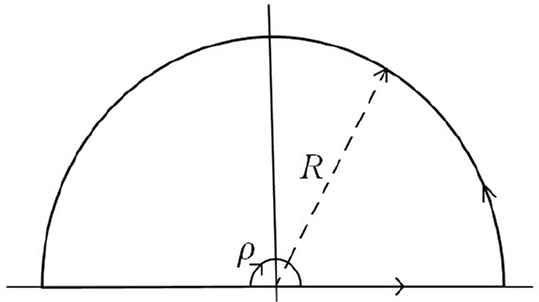
The Fourier transform (2.60) and its inverse Fourier transform map L2[x, ∞) onto L2[x, ∞) mutually continuously one-to-one, therefore K*(x, y) ∈ L2(x, ∞). Dividing equality (2.55) by s11(k):
The function s11(k) is analytical in the upper half-planeImk > 0 and has no zero there, then the function:
Multiply both sides of identity (2.61) by
Therefore, the function K*(x, y) satisfies the integral fundamental equation (2.41). From the uniqueness of a solution of Eq. (2.41), it follows that K*(x, y) = K(x, y). Then by (2.43) and (2.60) e*(k, x) ≡ e(k, x). Since the solution of equation (2.41) is the kernel of the transformation operator, then it satisfies Eq. (2.9). Due to the uniqueness of solution of Eq. (2.9), the solution K(x, y) of Eq. (2.41) is related to the potential by formula (2.48) and satisfies condition (2.49). Therefore, the restored potential (2.48) belongs to the class 𝒮. Thus, the Schrödinger equation (2.4) is restored with the potential (2.48) satisfying condition (2.49). In addition, the negative spectrum of the restored equation is absent. Thus, the first assertion is proved.
We proceed to prove the second assertion. Let s11(k) and s21(k), −∞ < k < ∞ be any given functions satisfying the sufficient conditions enumerated in Theorem 2.1. We prove that these given functions are the scattering data of the SP (2.1)–(2.2) with the restored potential belonging to the class 𝒮. In fact, consider the SP with the restored potential (2.48) satisfying condition (2.49). Let
Since the solutions K(x, y) and
For a sufficiently large positive x = x0, the integral operator in homogeneous equation (2.63) is a contracting operator in the space of functions bounded on the interval (x0, ∞). Hence, for x ≥ x0 and
For fixed x0 and y, Eq. (2.64) is a Volterra homogeneous, therefore
Then owing to uniqueness of expansion of a function in the Fourier integral:
Thus, the ratios:
The KdV equation (1.1) is derived from the Lax condition for compatibility of two systems:
The potential p(x, t) for every t > 0 belongs to the class 𝒮, therefore the systems (2.66) and (2.67) are compatible, i.e.,
The above equality will be referred to as the compatibility condition for systems (2.66) and (2.67). It is easy to verify that this compatibility condition is equivalent to the KdV equation (1.1). The boundary conditions (1.2) are satisfied if and only if the system (2.67) along the line x = 0 takes the form:
Upon differentiating equality (2.14) with respect to t, we have the equality:
Substituting matrix expressions Et and Wt into equality (2.69), using conditions (1.2), we derive the system of linear differential equations governing the time-dependence of s(k, t):
The time-dependence of the scattering matrix s(k, t) defined by system (2.70) implicitly depends on the time t. This is the main difference between the IBVP (1.1)–(1.2)–(1.3) and the Cauchy problem, therein lies the difficulty in passing from the Cauchy problem to this IBVP. The system (2.70) is undetermined, because the function px(0, t) entering coefficients of this system is unknown. In Sec. 3 we shall prove that the unknown object px(0, t) can be expressed through entries of the given s(k).
3. The self-conjugate problem
The system (2.68) describes the time-evolution of the eigenfunction for the boundary point x = 0. Using the linear change of dependent variables: Y (k, t) = J(k)ỹ(μ, t), we reduce (2.68) to the form:
Let β = −ik, then the matrix J in (3.1) coincides with the matrix T(k) defined by:
Thus, by virtue of the linear change of dependent variables given by (3.3), we lead system (3.2) into the system of first-order ordinary differential equations on the half-line:
Denote ỹ(μ, t) by y(μ, t) and consider the self-conjugate SP generated by system (3.4):
We also consider the problem for system (3.6) for real μ with boundary conditions at infinity:
Assume that the potential function px(0, t) in (3.5) satisfies the estimate:
The problems (3.6), (3.8) and (3.6)–(3.7) with the potential satisfying estimate (3.9) have been solved in [14]. Since the potential matrix (3.5) is a particular case of the potential self-conjugate matrix of the problem investigated in [14], then the following Propositions are deduced from corresponding assertions proved in [14] without proving.
Proposition 3.1.
The problem (3.6)–(3.7) has a unique bounded solution (y1(μ, t), y2(μ, t)) for real μ such that for any given number A(μ) there exists a unique number B(μ) defined from A(μ) so that the asymptotics (3.8) are satisfied. This solution has the representation:
Using condition (3.5), wherein the functions c1(t), c2(t) are pure imaginary functions, from the integral equations for kernels we obtain that the solutions Hjk(t, s), j, k = 1, 2 of these equations are real-valued functions, and
The kernel function H21(t, t + ξ) is related to the potential px(0, t) by the formula:
Proposition 3.2.
There exist the bounded Jost solutions
By an argument analogous to problem (3.6)–(3.7) on the half-line 0 ≤ t < ∞, for any t ≥ 0 we consider the problem generated by system (3.6) on a half-line t ≤ τ < ∞ with the boundary condition at τ = t:
Definition 3.1.
The one-to-one correspondence between numbers A(μ, t) and B(μ, t) determines the scattering function S(μ, t): S(μ, t)A(μ, t) = B(μ, t), −∞ < μ < ∞ for the SP generated by system (3.6) on the half-line: t ≤ τ < ∞ with condition (3.13).
By Definition 3.1 and using (3.10), (3.13), we derive the factorization of S(μ, t):
By virtue of estimate (3.11) and the self-conjugate property of matrix (3.5), the function H(t, ξ) is absolutely integrable with respect to ξ, the numerator 1 + H−(μ, t) and denominator 1 + H+(μ, t) of ratio (3.14) are different from zero and analytic in the half-planes Im μ ≤ 0 andIm μ ≥ 0, respectively. There exists an absolutely integrable with respect to ξ function K(t, ξ) such that
Furthermore, for any t ≥ 0 the scattering function S(μ, t) possesses the property:
Proposition 3.3.
For any t ≥ 0 the scattering functions S(μ, t) − 1 and S−1(μ, t) − 1 for the SP (3.6), (3.13) are the Fourier transformations:
Proposition 3.4.
There exists uniquely a solution φ(μ, t) = (φ1(μ, t), φ2(μ, t)) of (3.6) with the initial condition: φ1(μ, 0) = φ2(μ, 0) = 1. The function φ(μ, t) is entire analytic of μ, and:
Proposition 3.5.
For any t ≥ 0 the functions f(t, ξ) and g(t, ξ) defined by (3.18) and (3.19) are closely related to f(ξ) and g(ξ), respectively by the formula:
The functions f(−ξ) and g(ξ), ξ > 0 satisfy the estimate of the type (3.9):
Proposition 3.6.
For every fixed t ≥ 0 the following Fredholm system:
Proposition 3.7.
For the given function S(μ) to be the scattering function for the self-conjugate problem (3.6)–(3.7), it is necessary and sufficient that there exists a function S(μ, t) such that S(μ) = S(μ, 0) and
- 1.
the function S(μ, t) admits the factorization of the form (3.14);
- 2.
- 3.
To solve the inverse SP (3.6)–(3.7) for finding the unknown object px(0, t), we need to find the unknown scattering function S(μ) of this problem first. To find S(μ), we express the function S(μ) through known elements of the scattering matrix s(k) of the SP (2.1)–(2.2). This is the key step to recover the potential matrix (3.5), i.e., the system (3.6).
The matter is that the first SP (2.1), (2.2) and the second SP (3.6)–(3.7) are formulated on two different spectral planes. The first SP is considered on the k-plane, whereas the second SP is considered on the μ-plane, (μ = k3). To compare functions on the k-plane with those on the μ-plane, we use the conjugation contour. The contour Im μ = Imk3 = 0 splits into a system of rays The conjugation contour.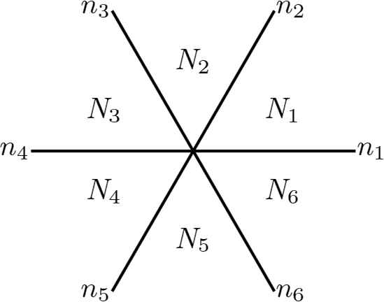
We compose the matrix functions ψ+(μ, t) and ψ−(μ, t) according to the rule:
Since the matrix functions
The functions s1(k, t) and s2(k, t) are defined in the half-planes Imk ≥ 0 and Imk ≤ 0, respectively. We compose the matrix functions Φ + and Φ − by columns of matrices (2.5) and (2.6) at x = 0 according to the rule:
Using the consistency condition for systems (2.66) and (2.67) in the quarter of the plane x ≥ 0, t ≥ 0, we calculate α(k, 0) and β(k, 0). In view of system (2.68) for the eigenfunction along the line x = 0 and the change of variables (3.3), this consistency condition means that the matrix functions T(k)ψ+(μ, t), T(k)ψ−(μ, t) defined on μ-plane and Φ +(k, 0, t), Φ −(k, 0, t) defined on k-plane must be consistent at the corner point (x, t) = (0, 0) for all values of k. Making use of this fact, we calculate α(k, 0) and β(k, 0) for k ∈ Nj, j = 1, 2, ...,6, [11]:
Using formula (3.21), (3.26) and (3.27), from (3.28)–(3.31) for t = 0, we get:
Here the coefficients α(k, 0), β(k, 0) are calculated by formulas (3.32)–(3.37):
Due to (2.20), from (3.40) we have the asymptotics as |k| → ∞:
Using the self-conjugate property of the SP (3.6)–(3.7) and (2.16), (2.19), (2.20) we get:
Hence, the found quantities D(μ), N(μ) and S(μ) satisfy all properties assembled in Proposition 3.4.
4. The time-evolution of s(k, t) and solution of the IBVP
The differential equations for functions s1(k, t) and s2(k, t) are derived from system (2.70) for columns of the matrix s(k, t):
Further, differentiating equality (3.28) with respect to t and taking into account that the matrix functions s(k, t) and
By comparison of the last equality with equality (4.1), using (3.28) for k ∈ N1 we derive the evolution equation:
Using (3.32), from (4.3) we obtain the explicit formulas for the coefficient (α(k, t), β(k, t)) :
Thus, the evolution in time t, t > 0 of s1(k, t) for k ∈ N1 is derived from (3.28) with this coefficient:
In the same way as in the previous case, by using (4.1), (4.2), (3.28)–(3.31) and (3.33)–(3.37), analogously derive:
Hence, the obtained columns s1(k, t) and s2(k, t) are expressible by expansion formulas (4.4)–(4.6) and (4.7)–(4.9), respectively in their sectors in terms of entries of s(k, 0) and fundamental solutions ψ±(μ, t) of system (2.70). The solutions Ψ ±(μ, t) are calculated from known conditions (1.2) and (1.3). The condition t ≥ 0 is important precisely here. Indeed, for t < 0 the functions s1(k, t) and s2(k, t) are therefore, no longer bounded at infinity of t.
We are now to solve the IBVP (1.1)–(1.3). By Theorems 2.1 and results presented in Secs. 3 and 4, this problem is reduced to that of solving the GLM time-dependent equation (2.41):
From the unique solvability of Eq. (2.41), it follows that for every t ≥ 0 the Eq. (4.10) has a unique solution in either L2[x, ∞) or L1[x, ∞). By condition (2.38) and Parseval’s relation, we find that ‖R‖L2 < 1 in L2[x, ∞). Consequently, Eq. (4.10) can be solved by the method of successive approximations. The solution of Eq. (4.10) may be represented as a convergent Neumann series:
The solution p(x, t) of the IBVP (1.1)–(1.3) is constructed by formula (2.11) expressed through the solution (4.12) of Eq. (4.10):
Hence, the solution (4.13) of Eq. (1.1) corresponding to solution (4.12) of Eq. (4.10) is determined by:
One can verify directly that the solution (4.14) satisfies Eq. (1.1) to any desired order in powers of R. The presentation (4.14) in formality is similar to that of the solution of the KdV equation with the positive coefficient of the dispersive term on the whole-line, that evolves from a purely continuous spectrum, [9].
By Theorem 2.1 the solution of Eq. (4.10) coincides with the kernel of the transformation operator of the SP (2.1)–(2.2) with potential (4.14). Hence, p(x, t) determined by (4.14) belongs to the class 𝒮, and therefore it satisfies condition (2.49).
Consider the asymptotic behaviour of s1(k, t) and s2(k, t) at infinity of time (t). Substituting (3.26) into (4.4), (4.6) and (4.8), using Propositions 3.2, and 3.4 gives:
Substituting (3.27) into (4.5), (4.7) and (4.9), using Propositions 3.2, and 3.4, gives:
From the obtained asymptotics it follows that
It is known that if the spectrum of Eq. (2.4) is purely continuous, then the asymptotic solution p as t → ∞ of the KdV equation on the whole line is still slowly varying wave train, oscillating about p = 0, (see [9]). Hence, the asymptotic solution (4.15) at infinity of t of the IBVP (1.1)–(1.3) is different from that of the KdV equation on the whole line.
5. Exact soliton-solutions of the Cauchy problem for the KdV equation
We consider the Cauchy problem for the KdV equation:
The Cauchy problem (5.1)–(5.2) is associated with the SP for the Schrödinger equation:
5.1. The direct and inverse SP (5.4)–(5.5)
The SP (5.4)–(5.5) with the potential p(x) satisfying condition (5.3) has been investigated in the works [6,7]. In the subsection 5.1 we recall the known results of this SP from these works and omit the proof.
Eq. (5.4) with the potential p(x) satisfying condition (5.3) has a solution e(ρ, x), which for each x ≥ 0 is a holomorphic function of ρ when
For each ρ0 > 0 Eq. (5.4) has a solution e1(ρ, x), which for each x ≥ 0 is holomorphic function of ρ in the domain |ρ| > ρ0,Imρ > 0, and satisfies the asymptotic condition as x → ∞:
The functions e(ρ, x), e(−ρ, x) and e(ρ, x), e1(ρ, x) form the fundamental systems of solutions of Eq. (5.4) and their Wronskians are equal to:
The solutions of Eq. (5.4) can be represented in the form:
Denote by ω(ρ, x) the solution of the eigenvalue problem generated by Eq. (5.4):
By virtue of (5.8) and (5.9), the solution of the problem (5.11)–(5.12) is represented in the form:
Differentiating the equality (5.14) with respect to x, using the initial condition (5.12), we have:
By L we mean the operator generated in the space L2[0, ∞) by Eq. (5.4) and boundary condition (5.5). The potential p(x) in the operator L is a real-valued function. Consider an eigenfunction Ω(ρ, x) of the operator L normalized in the following way:
By (5.13) and (5.14), the normalized eigenfunction Ω(ρ, x) is represented in the form:
The functions S(ρ) and S1(ρ) are called the scattering function and the reflection coefficient of the operator L, respectively.
Since the potential in Eq. (5.11) is a real-valued function satisfying estimate (5.3), then all the zeros ρj of the function e(ρ) are simple and lie on the imaginary axis, i.e., ρj = iμj, μj > ε0 > 0, j = 1,...,N. By virtue of this fact, using the expression (5.15), we calculate:
We introduce the function:
The integral (5.20) is applied to analytic function S(ρ) − 1 in the strip 0 < |Imρ| < ε0, therefore its value will not depend on η.
The function FS(x) like the scattering function S(ρ), is a spectral characteristic of the operator L on its continuous spectrum. While the functions fj(x) defined by (5.18) characterize the operator L on its point spectrum.
The scattering function S(ρ), the nonsingular numbers iμj,...,iμN and the normalization multipliers
The kernel K(x, y) from (5.10) satisfies the GLM equation:
Eq. (5.22) has a unique solution K(x, y), and the potential p(x) is recovered through the found solution by the equality [7]:
5.2. Non-scattering potentials
There exists a remarkable class of potentials, for which Eq. (5.22) can be solved exactly. These are non-scattering potentials on the half-line, for which the inverse Fourier transform FS(x) defined by (5.20) in the sense of generalized functions is equal to zero, [12]. Hence, in the class of non-scattering potentials the functions FS(x) and F(x) defined by (5.20) and (5.21), respectively, are
Our definition of non-scattering potential is similar to the definition of reflectionless of potentials, for which the reflection coefficient is identically zero [8].
Under the condition (5.24) Eq. (5.22) can be solved exactly. Indeed, the solution K(x, y) of this equation is to be sought in the form:
Substituting (5.25) into Eq. (5.22), after some simple transformations, we obtain a system of linear algebraic equations for Kj(x):
Let D(x) denote an N × N square matrix consisting of the elements:
From linear algebra, we know that the solution of the system (5.26) is
Since the potential p(x) is determined by K(x, x), then we calculate it with the help of (5.25):
Using the rule of differentiation of determinants, we find that the numerator in this expression is equal to the derivative of detD(x), because
The expression (5.28) completely describes the whole family of non-scattering potentials.
5.3. The time-dependence of the reflection coefficient
It is known that the KdV equation (5.1) is identical to the equation defined by the Lax representation [8]:
The potential p(x, t) in the operator L(t) is called isospectral if the spectrum of L(t) is invariant with t, i.e.,
Differentiating Eq. (5.30) with respect to t and using (5.31), we have:
It follows from (5.32) that the Lax representation (5.29) for the nontrivial eigenfunction Ω holds if and only if
Lemma 5.1.
If the potential p(x, t) in the operator L(t) satisfies the KdV equation (5.1), then the time-dependence of the normalization eigenfunction (5.16) is defined by the evolution equation:
Proof.
Let the potential p(x, t) in L(t) satisfy the KdV equation (5.1), then the time-dependence of the normalized eigenfunction (5.16) is given by the evolution equation (5.31). Using (5.29), we write Eq. (5.31) in the form:
Due to (5.6) and (5.7) the normalization eigenfunction (5.16) obeys the asymptotic condition as x → ∞:
Since p(x, t) is a solution of the KdV equation (5.1), then the potential p(x, t) is a isospectral potential. Using this fact and (5.3), (5.36), in (5.35) letting x tend to ∞, we find
Hence, γ = 4iρ3, and the time-dependence of the functions Ω and S1 defined by evolution equations (5.33) and (5.34) are deduced from (5.31) and (5.37), respectively. The lemma is proved.
The Lemma 5.1 enables us to find the time-dependent potential p(x, t) in the class of non-scattering potentials. In fact, the time-dependent matrix D(x;t) is obtained from the matrix D(x) given by (5.27) with the help of the following substitution:
The formulas (5.28) and (5.38) give exact soliton-solutions of the KdV equation (5.1) in the class of non-scattering potentials:
The soliton-solution (5.39) of the KdV equation (5.1) is constructed from the non-scattering data s of the associated scattering problem (5.4)–(5.5):
Theorem 5.1.
Let the function p(x) in the operator L be an isospectral non-scattering potential which is a real-valued continuous function satisfying the estimate (5.3). Then the normalization multipliers
5.4. An example
Example. Let the non-scattering data (5.41) consist of two simple poles ρ1 = iμ1 and ρ2 = iμ2, μ1 > μ2 > 0. In this case the elements Djn(x, t) of the matrix D(x, t) are calculated by (5.39) and (5.40):
Putting
The non-scattering real-valued potential p(x, t) is calculated by formulas (5.39)–(5.40)
It is easy to verify that
Hence,
Using (5.45), (5.46) and (5.48), we calculate:
The explicit soliton-solution p(x, t) of the KdV equation (5.1) with two bound states is obtained from (5.47), using (5.48), (5.49) and (5.50):
Thus, p(x, t) represents the nonlinear superposition of two forms, one traveling with speed
We suppose that μ1 > μ2, then from (5.43)–(5.44) it follows that for every x:
While in the region of x, where η is about one and ξ is very positive, we obtain:
That is, for very large negative t the solution looks like two solitary pulses, the large one to the left of the small one.
After a long time, when t is large positive, it follows from (5.43)–(5.44) that for every x:
While if ξ is order one, and η very large positive, then
That is after a long time the large solitary pulse is to the right of the small solitary pulse. They have coalesced and reemerged with their shaped unscathed. The only remnant of the interaction is the phase shift Two soliton-solution of the KdV equation (5.1) with two bound states at the four successive moments of time t = t0, t1, t2 and t3.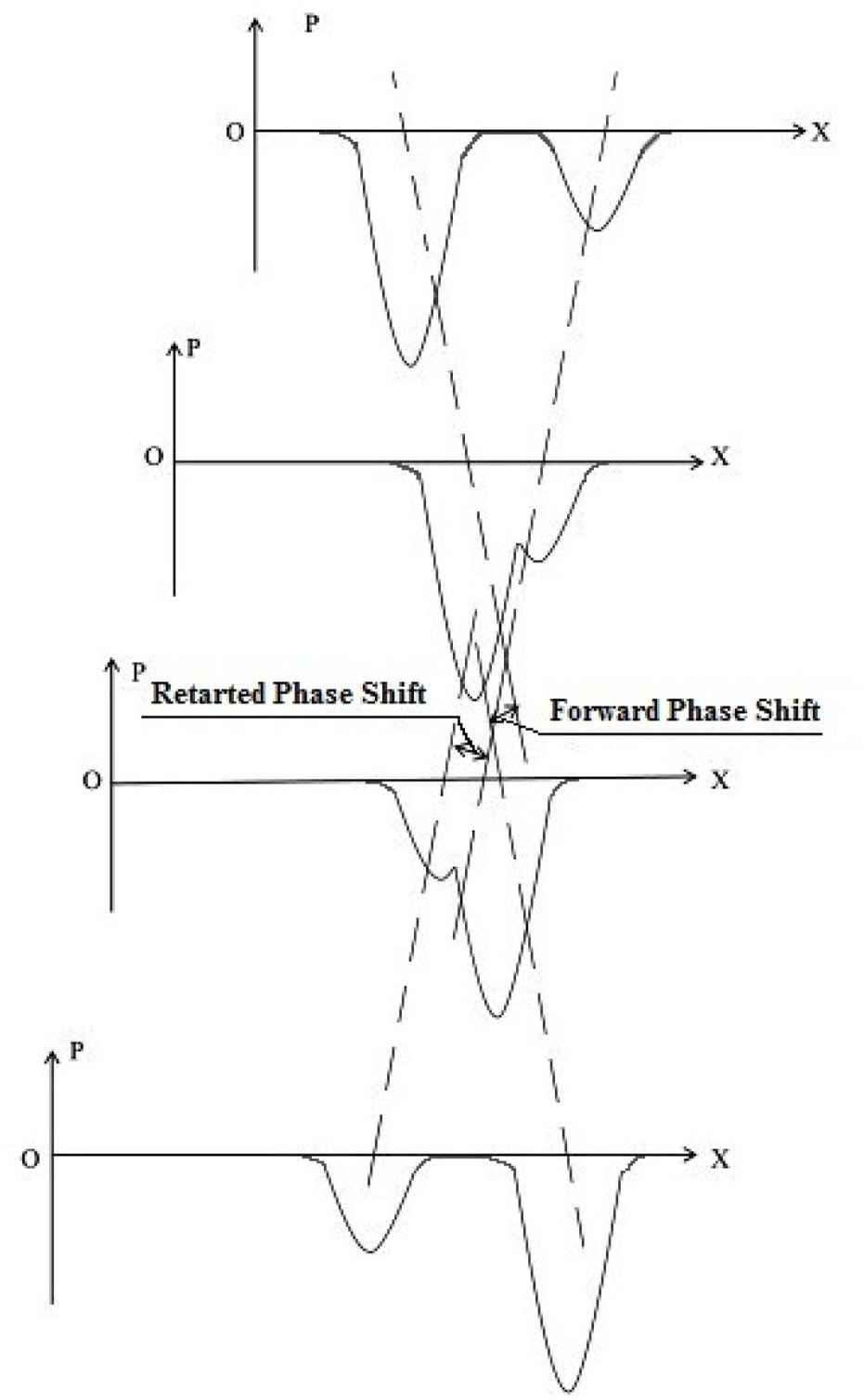
In general, the non-scattering solution with N bound states has a similar behavior. In this case the non-scattering data (5.41) consist of N simple poles: ρj = iμj, μj > 0, j = 1,...,N. With N bound states the solution resembles the superposition of N solitary pulses whose speeds and amplitudes are determined by the positive values μj, j = 1,...,N. The solitary pulses emerge unscathed from interaction except for a phase shift given by the sum of phase shifts from all possible pairwise interactions.
6. Conclusions
By Propositions 3.6, 3.7 and formulas (3.42)–(3.44), the self-conjugate matrix (3.5) is found uniquely from the known conditions (1.2) and (1.3). Then the time-dependence of s(k, t) is derived by (4.4)–(4.9). The known function
By Theorem 5.1 the non-scattering potential (5.39) constructed from the non-scattering data (5.41) of the scattering problem (5.4)–(5.5) describes the whole family of non-scattering potentials which are soliton-solutions of the Cauchy problem for the KdV equation (5.1).
Acknowledgments
This work has been supported by the Vietnam National Foundation for Science and Technology Development (NAFOSTED) under grant number 107.03-2015.31.
References
Cite this article
TY  - JOUR
AU  - Pham Loi Vu
PY  - 2021
DA  - 2021/01/06
TI  - The description of reflection coefficients of the scattering problems for finding solutions of the Korteweg–de Vries equations
JO  - Journal of Nonlinear Mathematical Physics
SP  - 399
EP  - 432
VL  - 25
IS  - 3
SN  - 1776-0852
UR  - https://doi.org/10.1080/14029251.2018.1494777
DO  - 10.1080/14029251.2018.1494777
ID  - Vu2021
ER  -