
Cusped solitary wave with algebraic decay governed by the equation for surface waves of moderate amplitude
- DOI
- 10.1080/14029251.2020.1700632How to use a DOI?
- Keywords
- Cusped solitary wave; Algebraic decay; Free surface; Shallow water; Moderate amplitude
- Abstract
The existence of a new type of cusped solitary wave, which decays algebraically at infinity, for a nonlinear equation modeling the free surface evolution of moderate amplitude waves in shallow water is established by employing qualitative analysis for differential equations. Furthermore, the exact parametric representation as well as its planar graph for such type of wave is also given.
- Copyright
- © 2020 The Authors. Published by Atlantis and Taylor & Francis
- Open Access
- This is an open access article distributed under the CC BY-NC 4.0 license (http://creativecommons.org/licenses/by-nc/4.0/).
1. Introduction
The nonlinear evolution equation
As shown in [2], Eq. (1.1) approximates the governing equation to the same order as the Camassa-Holm (CH) equation, which models the horizontal fluid velocity at a certain depth beneath the fluid [8]. The great interest in the equations describing the moderate amplitude waves (e.g., the CH equation), lies in the fact that they exhibit a wider range of nonlinear phenomena, such as wave breaking and solitary waves with singularities, which the model equations derived within the small amplitude shallow water regime (e.g., the KdV equation) do not have, despite the fact that the governing equations for irrotational waves do admit peaked traveling waves (periodic, as well as solitary), namely the celebrated Stokes waves of greatest height, see [4, 5, 25] for example. It is shown in [3] that unlike the KdV and CH equations, Eq. (1.1) does not have a bi-Hamiltonian integrable structure. The local well-posedness results in Sobolev space for the initial value problem associated to Eq. (1.1) on the line and on the unit circle were reported in [17, 20, 27] and in [21], respectively. Further work on the well-posedness of Eq. (1.1) has been done in Besov space [24]. Moreover, some results on its wave breaking, global conservative solutions, low regularity solutions and continuity and persistence properties of strong solutions can be found in [2,19,21,22,26,27,29]. Eq. (1.1) has been shown to admit various kinds of traveling wave solutions, including smooth solitary wave, compacted solitary wave, cusped solitary wave, and smooth, peaked and cusped periodic wave solutions [9,10,12,28]. Further, it is proved that the smooth solitary waves are orbitally stable in [23] and that all symmetric waves are traveling waves in [11] for this equation.
In the present paper, we will use qualitative analysis method for differential equations, which is proposed by Lenells [15, 16], to solve Eq. (1.1). We prove that Eq. (1.1) admits a type of cusped solitary wave featured by decaying to zero algebraically at infinity. Such type of cusped solitary wave is different from those with exponential decay appeared in the former literature and thus is new for Eq. (1.1). Our work may help people to understand deeply the described physical process and possible applications of Eq. (1.1).
The remainder of paper is organized as follows. In Sec. 2, we prove the existence of cusped solitary wave with algebraic decay to Eq. (1.1) based on a weak formulation of Eq. (1.1). In Sec. 3, we give the exact parametric representation of such type of cusped solitary wave as well as its planar graph.
2. Existence of cusped solitary wave with algebraic decay
For a traveling wave solution u(t, x) = ϕ(x − ct), with c representing the constant wave velocity, Eq. (1.1) takes the form
Now we give the definition of solitary waves to Eq. (1.1).
Definition 2.1.
A solitary wave to Eq. (1.1) is a nontrivial traveling wave solution to Eq. (1.1) of the form ϕ(x − ct) ∈ H1(ℝ) with c ∈ ℝ and ϕ vanishing at infinity along with the first and second derivatives of ϕ.
Taking account of ϕ(x), ϕx(x) and ϕxx(x) → 0 as |x| → ∞, integration of Eq. (2.1) over (−∞, x] leads to
To deal with the regularity of the solitary waves, we give the following lemma, which is inspired by the study of traveling waves of Camassa-Holm equation [15].
Lemma 2.1.
Assume that ϕ is a solitary wave to Eq. (1.1). Then we have
Therefore
Proof.
Let ψ = ϕ − ρ and denote
Thus p(ψ) is a polynomial in ψ and then Eq. (2.3) can be written as
From the assumption, it follows that
For k ≥ 3 the right-hand side of (2.7) is in
Thus (2.4) holds for j = 1. Next, we assume that
Then for k ≥ 2j we have
Also we have ψk−2 p(ψ) ∈ Cj−1(ℝ). Therefore the right-hand side of (2.7) is in Cj−2(ℝ). Hence, in view of the relation ψ = ϕ − ρ, by induction on j, we know (2.4) holds.
Furthermore, it follows from (2.8) that
This implies that ψx ∈ C(ℝ \ ψ−1(0)) and thus ψ ∈ C1(ℝ \ ψ−1(0)). Now, we assume that ψ ∈ Cj(ℝ \ ψ−1(0)) for j ≥ 1. Then for k ≥ 2j+1, we have ψk ∈ Cj+1(ℝ). Thus
Setting x0 = min{x : ϕ(x) = ρ}, then we have x0 ≤ +∞. In view of Lemma 2.1, it follows that a solitary wave ϕ is smooth on (−∞, x0) and hence Eq. (2.3) holds pointwise on (−∞, x0). Therefore we may multiply both sides of Eq. (2.3) by 2ϕx and integrate on (−∞, x0) for x < x0 to get
We notice that F(ϕ) ≥ 0 if ϕ is a solution to Eq. (2.9).
Remark 2.1
As has been already pointed out in [15], a continuous function ϕ is said to have a cusp at x0 if ϕ is smooth locally on both sides of x0 and limx↑x0 ϕx(x) = −limx↓x0 ϕx(x) = ±∞. A solitary wave to Eq. (1.1) with a cusp on its crest or trough is called a cusped solitary wave. In addition, it should be pointed out that cusped waves are also relevant for the governing equations for water waves, since the limiting form of the Gerstner waves is a cycloidal profile with upward cusps, see [3, 13] for the case of gravity water waves and [6, 7, 18] for equatorial waves.
To determine the cusped solitary waves to Eq. (1.1), we also need the following lemma.
Lemma 2.2
The solution to Eq. (2.9) has the following asymptotic properties:
- (i)
If F(ϕ) has a simple pole at ρ, where ϕ(x0) = ρ, then
for some constant α, thus ϕ has a cusp. - (ii)
If ϕ approaches a triple zero m of F(ϕ) so that F(m) = F′(m) = F″(m) = 0, F′″(m) ≠ 0, then
for some constant β. Thus ϕ → m algebraically as x → ∞.
Proof.
Since the proof of (i) can be found in [15], then here we only consider the proof of (ii). Since m is a triple zero of F(ϕ), then it follows from (2.9) that
Furthermore, we have
Since
Integration gives
Based on the above derivation, now we give the following theorem on existence of cusped solitary wave with algebraic decay to Eq. (1.1).
Theorem 2.1.
If c = 1, then Eq. (1.1) admits an anti-cusped solitary wave ϕ < 0 with minx∈ℝ ϕ(x) = −1/7 and an algebraic decay to zero at infinity
Proof.
If c = 1, then Eq. (2.9) becomes
Hence we know that ϕ(x) < 0 near −∞. Since ϕ(x) → 0 as x → −∞, there exists some
It is easy to see that
Thus F1(ϕ) decreases for ϕ ∈ (−ε, 0). Since
Moreover, since ϕ = 0 is the triple zero of F1(ϕ) and F″′1(0) = −6, then we know from (ii) of Lemma 2.2 that (2.13) holds.
3. Expression of cusped solitary wave with algebraic decay
In this section we turn our focus to finding the parametric presentation of anti-cusped solitary wave for c = 1, whose existence is guaranteed by Theorem 2.1. We will use some symbols on the elliptic functions and elliptic integrals, see [1]. sn(·, k), cn(·, k) and dn(·, k) are Jacobian elliptic functions with the modulus k. cn−1(u, k) is the inverse function of cn(u, k). E(·, k) is the Legendre’s incomplete elliptic integral of the second kind.
Since ϕ is negative, even with respect to
The substitution of
Inserting (3.3) into (3.2) and solving the resulting equation with the initial value
Thus we obtain the exact anti-cusped solitary wave of parametric form with algebraic decay for c = 1 to Eq. (1.1) as follows:
The profile of (3.4) with
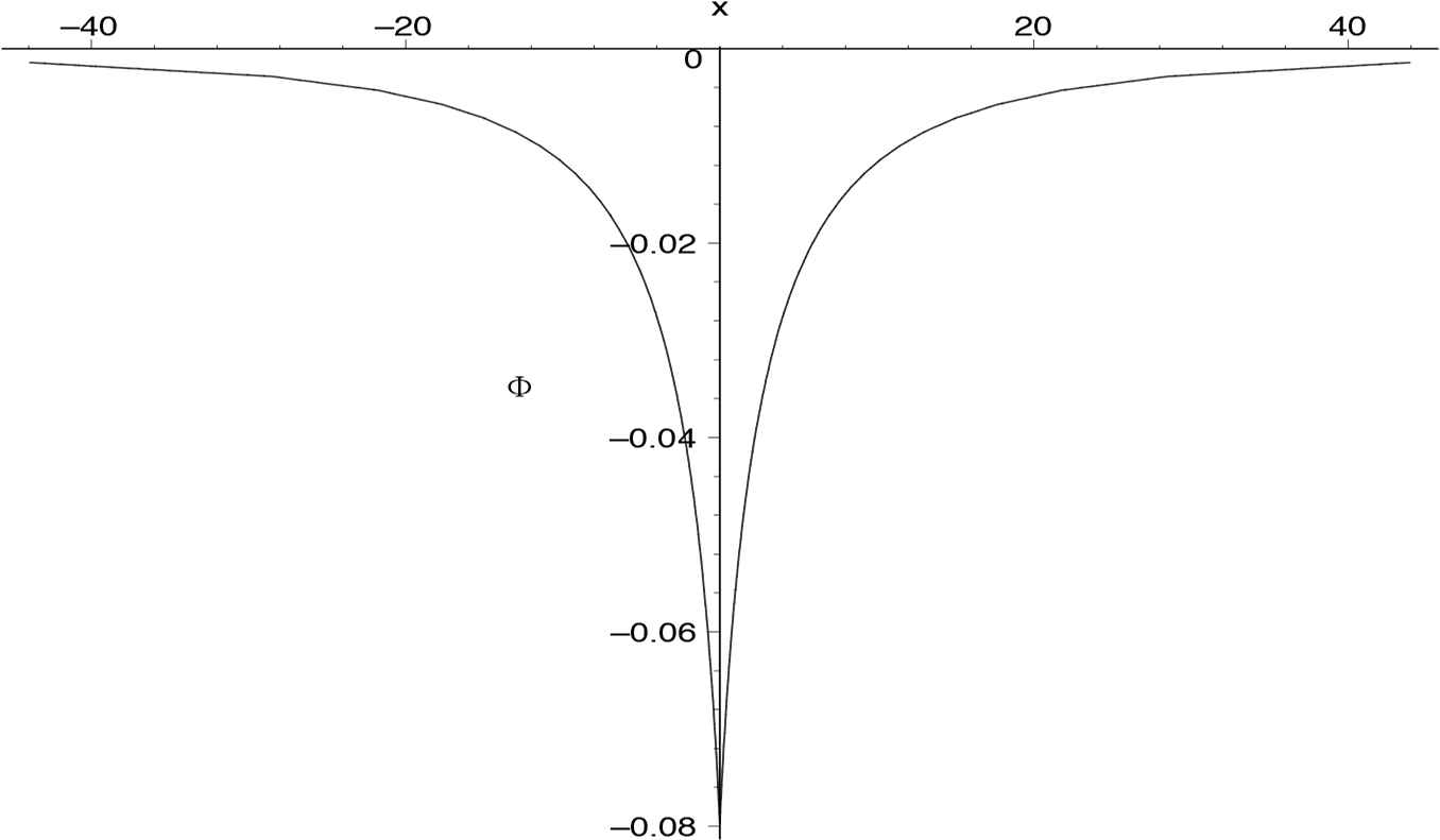
The planar graph of anti-cusped solitary wave.
Acknowledgments
The authors would like to thank the anonymous referee for the careful reading of the paper and many constructive comments and suggestions which have helped us to improve it. This work was done while the author was a visiting scholar at the University of Connecticut. The authors would like to thank the professor Guozhen Lu for his encouragement and help. This research was supported by the National Natural Science Foundation of China (No.10872080).
References
Cite this article
TY  - JOUR
AU  - Bo Jiang
AU  - Youming Zhou
PY  - 2020
DA  - 2020/01/27
TI  - Cusped solitary wave with algebraic decay governed by the equation for surface waves of moderate amplitude
JO  - Journal of Nonlinear Mathematical Physics
SP  - 219
EP  - 226
VL  - 27
IS  - 2
SN  - 1776-0852
UR  - https://doi.org/10.1080/14029251.2020.1700632
DO  - 10.1080/14029251.2020.1700632
ID  - Jiang2020
ER  -