
On the global dynamics of a three-dimensional forced-damped differential system
- DOI
- 10.1080/14029251.2020.1757232How to use a DOI?
- Keywords
- Global dynamics; Poincaré compactification; forced-damped system; invariant algebraic curve; invariant
- Abstract
In this paper by using the Poincaré compactification of ℝ3 we make a global analysis of the model x′ = −ax + y + yz, y′ = x − ay + bxz, z′ = cz − bxy. In particular we give the complete description of its dynamics on the infinity sphere. For a + c = 0 or b = 1 this system has invariants. For these values of the parameters we provide the global phase portrait of the system in the Poincaré ball. We also describe the α and ω-limit sets of its orbits in the Poincaré ball.
- Copyright
- © 2020 The Authors. Published by Atlantis and Taylor & Francis
- Open Access
- This is an open access article distributed under the CC BY-NC 4.0 license (http://creativecommons.org/licenses/by-nc/4.0/).
1. Introduction and statement of the main results
We consider the autonomous polynomial differential system
The integrability of system (1.1) has been studied in [4] where the authors give the description of all the invariant algebraic curves of the system. Let U be an open subset of ℝ3. A first integral H : U → ℝ of system (1.1) is a non-locally constant function which is constant on the trajectories of the system.
We say that two C1 functions H1,H2 : U → ℝ are independent on U if the 2 × 3 matrix ∂ (H1,H2)/∂(x,y,z) has rank 2 at all points (x,y,z) ∈ U except, perhaps, on a subset of zero Lebesgue measure. System (1.1) is completely integrable if it has two independent first integrals. If a system is completely integrable then we can obtain its global phase portrait simply by performing the intersection of the level sets of its first integrals. As far as we know the notion of a completely integrable differential system is due to A. Russell [11].
A function I(x,y,z,t) is an invariant of system (1.1) if dI/dt = 0 on the trajectories of the system, that is, an invariant is a first integral which depends on the time. The following result was proved in [4].
Theorem 1.1.
The following statements hold for system (1.1).
- 1.
If c = a = 0 and b = 1, it is completely integrable with the two independent first integrals H0 = x2 + (z + 1)2 and H1 = x2 − y2.
- 2.
If b = 1, a = 0 and c ≠ 0, it has the first integral H1 = x2 − y2.
- 3.
If b = 1 and a ≠ 0 it has the invariant I1 = H1e2at = (x2 − y2)e2at.
- 4.
If c = −a with a ≠ 0 it has the invariant I2 = (b(x2 − y2 − z2) + z2)e2at.
Theorem 1.1 will be used in the following sections for studying the global dynamics of system (1.1) having a first integral or an invariant. As any polynomial differential system, system (1.1) can be extended to an analytic system on a closed ball of radius one, whose interior is diffeomorphic to ℝ3 and its invariant boundary, a two-dimensional sphere 𝕊2 plays the role of the infinity of ℝ3. This ball will be denoted by B and called the Poincaré ball, due to the fact that the technique for doing so is the Poincaré compactification, which is described in detail in [1] (in fact in that paper the compactification is done for ℝn, and Poincaré in [10] did it in ℝ2).
Two polynomial vector fields are said to be topologically equivalent if there exists a homeomorphism on the closed Poincaré ball carrying orbits of the flow induced on the Poincaré ball by the first vector field into orbits of the flow induced in the Poincaré ball by the second vector field preserving or reversing the orientation of all the orbits.
By using this compactification technique for the dynamics of system (1.1), we can prove the next result.
Theorem 1.2.
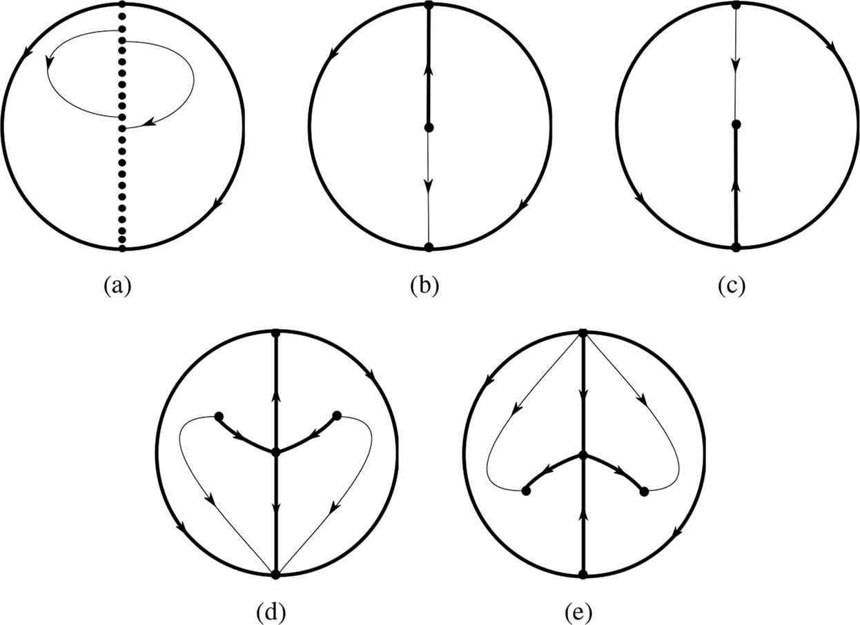
For all values of the parameters a, b, c ∈ ℝ with b > 0, the phase portrait of system (1.1) on the sphere at infinity, 𝕊2, is topologically equivalent to that of Figure 1. In that figure we can see that there exist four centers at the positive and negative endpoints of the x- and y-axis and two hyperbolic saddles at the positive and negative endpoints of the z-axis.
Note that the dynamics at infinity does not depend on the parameter values.
Now we continue the study of the dynamics of system (1.1) for the values of the parameters in Theorem 1.1. that is when b = 1 or a + c = 0 with a ≠ 0 (and b ≠ 1). We provide the description of the global dynamics of this polynomial differential system in its compactification on the Poincaré ball and we describe the α- and ω-limit sets of all orbits of system (1.1) for some values of the parameters.
Theorem 1.3.
The dynamics of the three-dimensional forced-damped differential system (1.1) in the Poincaré ball under the four assumptions given in the statement of Theorem 1.1 are described in section 4.
The paper is organized as follows. In section 2 we summarize several preliminary results of system (1.1). In section 3 we prove Theorem 1.2 by means of the Poincaré compactification technique, and in section 4 we prove Theorem 1.3.
2. Preliminaries
Lemma 2.1.
If ϕ(t) = (x(t),y(t),v(t)) is a trajectory of the compactified system (1.1) with a ≠ 0 and c = −a, or a ≠ 0 and b = 1, then its α-limit set α(ϕ) and its ω-limit set ω(ϕ) are contained in the closure in the Poincaré ball of the sets {H1 = x2 − y2 = 0} when b = 1, and {H2 = b(x2 − y2 − z2) + z2 = 0} when c = −a ≠ 0 (see Theorem 1.1).
Proof.
Assume first that a > 0. Let q1 ∈ ω(ϕ). Then there exists a sequence {tn} such that tn → ∞ and ϕ(tn) → q1. Thus, by statements 4 and 5 of Theorem 1.1 we have
Suppose now that q2 ∈ α(ϕ). Then there exists a sequence {tn} such that tn → −∞ and ϕ(tn) → q2. Hence
Thus the constant κ is zero and then Hi(ϕ(tn)) · e2atn → 0. This implies that Hi(ϕ(tn)) → 0 and so q2 is in the closure in the Poincaré ball of the set {Hi = 0}.
The case a < 0 can be done in the same manner reverting the roles of q1 and q2.
Lemma 2.2.
For all values of the parameters a, b, c the z-axis is an invariant set of system (1.1). The flow restricted to this invariant straight line is as follows: if c < 0 the origin (0,0,0) is a global attractor. If c > 0 then the origin is a global repeller. If c = 0 all points in the z-axis are singular.
Proof.
It follows directly from system (1.1).
Now we study the finite singular points whenever a ≠ 0 and c = −a or ac ≠ 0 and b = 1. Let p be a hyperbolic singular point of system (1.1) whose Jacobian matrix has k eigenvalues with negative real part. Then its stability index is k. Of course, 0 ⩽ k ⩽ 3. The topology index of p is given by (−1)k (see Theorem 8.1 of [5]).
Lemma 2.3.
Consider system (1.1) with b = 1 and ac ≠ 0.
- 1.
If c < 0 and a > 1 the unique singular point is the origin which has stability index 3 (an attractor).
- 2.
If c < 0 and a = 1 the unique singular point is the origin whose eigenvalues of its Jacobian matrix are −2, 0, c.
- 3.
If c < 0 and a ∈ (−1,1) it has three singular points: the origin and
- 4.
If c < 0 and a = −1 it has three singular points: the origin whose eigenvalues of its Jacobian matrix are 2, 0, c, and the two points (
- 5.
If c < 0 and a < −1 it has five singular points: the origin which has stability index 1,
- 6.
If c > 0 and a > 1 it has five singular points which are the origin (with stability index two),
- 7.
If c > 0 and a = 1 it has two singular points which are the origin (whose eigenvalues of its Jacobian matrix are −2, 0, c and (
- 8.
If c > 0 and a ∈ (−1,1) it has three singular points which are the origin and
- 9.
If c > 0 and a = −1 it has the origin as its unique singular point whose eigenvalues of its Jacobian matrix are 2, 0, c.
- 10.
If c > 0 and a < −1 it has the origin as its unique singular point which has stability index zero (a repeller).
Proof.
The proof of the lemma follows by direct calculations.
Lemma 2.4.
Consider system (1.1) with c = −a, a ≠ 0 and b ≠ 1:
- 1.
If a > 1 it has the origin as its unique singular point which has stability index three (an attractor).
- 2.
If a = 1 it has the origin as its unique singular point whose eigenvalues of its Jacobian matrix are −2, −1, 0.
- 3.
If a ∈ (−1,1) it has three singular points which are the origin and
withAll three points have stability index two when a ∈ (0,1) and stability index one when a ∈ (−1,0).
- 4.
If a = −1 it has the origin as its unique singular point whose eigenvalues of its Jacobian matrix are 2, 1, 0.
- 5.
If a < −1 it has the origin as its unique singular point which has stability index zero (a repeller).
Proof.
The proof of the lemma follows by direct computations.
3. Proof of Theorem 1.2
For studying the infinity of the Poincaré ball B we analyze the flow at infinity for the local charts U1, U2 and U3 (see [1]), as well as in the local charts V1, V2 and V3.
3.1. Study of the infinity in the local charts U1 and V1
The Poincaré compactification p(X) of system (1.1) in the local chart U1 is given by
Note that the unique singular point of system (3.1) on z3 = 0 is the origin (0,0,0) and the eigenvalues of the linear part of the system at this point are ±ib, and 0. System (3.1) restricted to z3 = 0 (because this corresponds to the sphere at infinity) reduces to
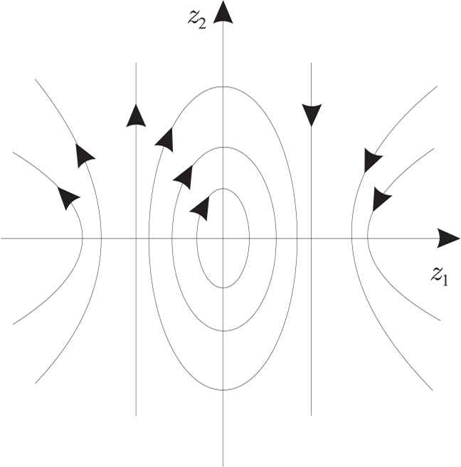
Phase portrait of system (3.2).
3.2. Study of the infinity in the local charts U2 and V2
The expression of the Poincaré compactification in the local chart U2 of system (1.1) writes as
Taking z3 = 0, system (3.3) becomes
Again we observe that the flow on the local chart V2 is the same as the flow on the local chart U2 reversing the time, because the compactified vector field p(X) in V2 coincides with the vector field p(X) in U2 multiplied by −1.
3.3. Study of the infinity in the local charts U3 and V3
The expression of the Poincaré compactification of system (1.1) in the local chart U3 is given by
If z3 = 0 the unique singular point of system (3.5) is p = (0,0,0). We want to study the local flow of this system around p. The eigenvalues of the linear part at p are
Proof.
[Proof of Theorem 1.2] Considering the analysis made in the previous sub-sections we obtain the phase portrait of system (1.1) on the sphere at infinity: the system has four centers, localized at the endpoints of the x and y-axis, and two saddles localized at the endpoints of the z-axis (see Figure 1). Moreover, the orbits of the system may come and go to infinity along a one-dimensional center manifold of these saddle points, depending on the sign of the parameter c. The dynamics near the center at infinity is more complex, due to the periodic orbits.
Phase portrait of system (1.1) on the sphere at infinity.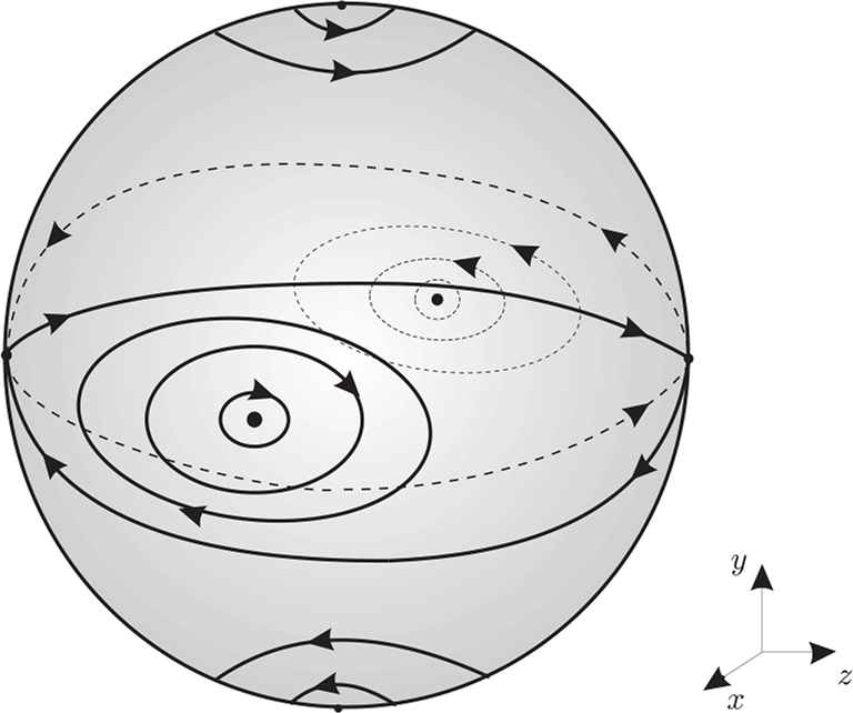
4. Proof of Theorem 1.3
In this section we prove Theorem 1.3. We consider the invariants and first integrals given in Theorem 1.1 and how the surfaces end in the Poincaré sphere at infinity.
4.1. Case b = 1, a = c = 0
In this case system (1.1) is completely integrable. There are three straight lines filled of singularities (0,0,z), (x,0,−1) and (0,y,−1). The endpoints of the straight line (0,0,z) on the Poincaré sphere are (0,0,±1), the endpoints of the straight line (x,0,1) are (±1,0,0), and the endpoints of the straight line (0,y,−1) are (0,±1,0). According to the introduction the trajectories are in the intersection of the elliptic cylinder x2 + (z + 1)2 = c1 with the hyperbolic cylinder x2 − y2 = c2, where c1 ⩾ 0 and c2 ∈ ℝ. The intersection produces families of periodic orbits, and for c1 = c2 the intersection occurs on the straight line (x,0,−1).
4.2. Case b = 1, a = 0, c ≠ 0
In this case H1 = x2 − y2 is a first integral. We study the dynamics of system (1.1) restricted to the hyperbolic cylinders x2 − y2 = ±r2 if r ≠ 0, and on the planes (x − y)(x + y) = 0 for r = 0.
For r = 0 the level is formed by two invariant planes with endpoints being the separatrices of the saddles on the Poincaré sphere. In the plane y = −x system (1.1) becomes
If c < 0 the unique singular point of system (4.1) is the origin (0,0) which is a stable node.
Now we study the phase portrait in a neighborhood of the infinity. Since system (4.1) is defined in ℝ2 we study it doing the Poincaré compactification in the Poincaré disc, see for more details on the Poincaré disc, Chapter 5 of [3]. System (4.1) in the local chart U1 given by the Poincaré compactification is
Note that there are no infinite singular points on U1. On the other hand system (4.1) on the local chart U2 is
We study the origin of U2 which is a semi-hyperbolic singular point. Applying Theorem 2.19 of [3] we get that it is a saddle-node with central manifold on z1 = 0 (where the flow is increasing), and the stable separatrices are located on z2 = 0. Since system (4.1) has degree two, the local phase portrait on V2 have the opposite stability.
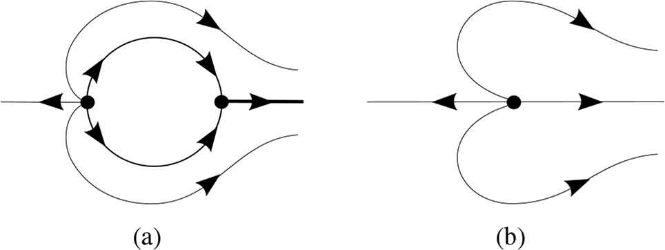
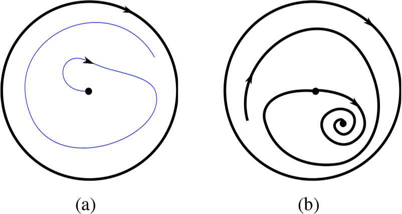
Since the unique finite singular point of system (4.1) is the origin and the straight line x = 0 is invariant, the system has no limit cycles. In short, by the Poincaré-Bendixson theorem (see for instance Corollary 1.30 of [3]) the unstable separatrix of the saddle-node at the origin of U2 has ω-limit the finite singular point (0,0). See the phase portrait in the Poincaré disc of Figure 3(a).
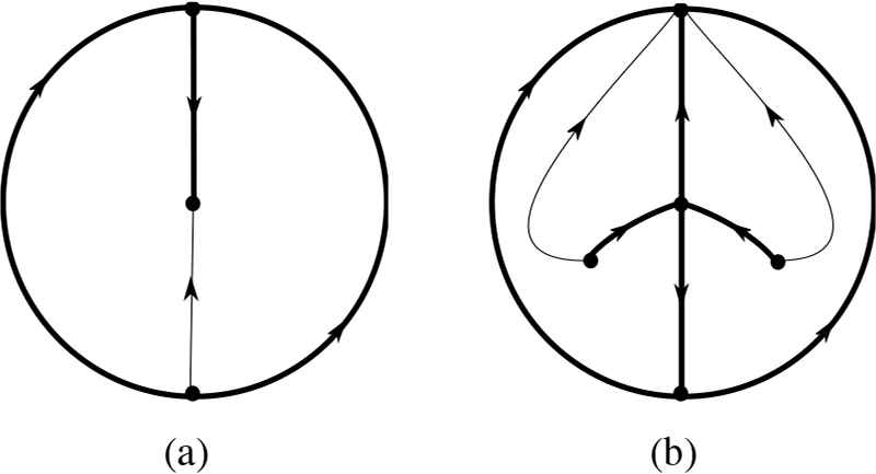
Global phase portrait of system (4.1) for b = 1 and a = 0. (a): with c < 0, (b): with c > 0.
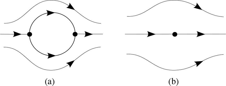
If c > 0 there are two more singular points beyond the origin. The origin is a saddle in this case and the two new singular points are unstable nodes if c − 8 ⩾ 0, or unstable foci if c − 8 < 0. Proceeding in a similar way to the case c < 0, the unique infinite singular points are the origins of U2 and V2, which are saddle-nodes, but now the nodal part of the saddle-node is in U2, see Figure 3(b). The unstable separatrices of the origin are contained in the straight line x = 0 and they go to the origins of U2 and V2. By the Poincaré-Bendixson theorem the stable separatrices at the origin have α-limit at the repeller nodes (or foci) in the finite region. This completes the global phase portrait of system (4.1) for c > 0, see Figure 3(b).
In the plane y = x system (1.1) becomes
Note that system (4.2) is the same as system (4.1) doing the reparameterization of the time t → −t and changing the parameter c by −c. This implies that the global phase portraits of system (4.2) are topologically equivalent to the ones shown in Figure 3.
The straight line (0,0,z) (intersection of the planes y = −x and y = x) is invariant with its points having (0,0,0) as their ω-limit.
For r ≠ 0 we have a pair of hyperbolic cylinders. System (1.1) restricted to the hyperbolic cylinder x2 − y2 = r2, r ≠ 0, (taking
Note that system (4.3) and system (4.4) are the same doing the change c → −c and reparameterizing the time by t → −t. Then it is sufficient to analyse the phase portraits of system (4.3).
System (4.3) has a unique finite singular point which is a stable node or stable focus if c < 0, and an unstable node or unstable focus if c > 0.
There are no infinite singular points in the local chart U1. In the local chart U2 system (4.3) becomes
The origin of system (4.5) is an infinite singular point whose eigenvalues are 0 and 1. Since it is semi-hyperbolic it can be a saddle, a node or a saddle-node. Considering that the sum of the indices of all singular points on the Poincaré sphere is 2 by the Poincaré-Hopf Theorem (see Theorem 6.30 of [3]), and since the finite singular points are two nodes (or two foci), it holds that the origin in U2 must be a saddle-node. From (4.5) we have
Doing the change of time
Since the divergence of this system is
Note that by the Poincaré-Bendixson theorem the unstable separatrix coming from the origin of U2 must go to the finite attractor. In summary, the global phase portrait for c > 0 (for c < 0 is the same reversing the direction of the orbits) is the one of Figure 4.
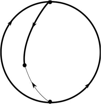
Global phase portrait of system (4.3).
Furthermore system (1.1) restricted to the hyperbolic cylinder x2 − y2 = −r2, r ≠ 0, (taking
Systems (4.6) and (4.7) coincide with systems (4.3) and (4.4), respectively, doing the change of variables (y,z) → (x,z). Then their phase portraits are the same than the one of Figure 4.
The phase portraits in the Poincaré ball for this case can be obtained using the previous information together with Figure 1.
4.3. Case b = 1, a ≠ 0
The planes x = ±y are invariant by the flow of system (1.1). The boundary at infinity of the invariant planes y = ±x coincide exactly with the heteroclinic cycles of the saddles at infinity.
Taking y = x system (1.1) becomes
The infinite singular points of system (4.8) are the same than the infinite singular points of system (4.1).
If c = 0, system (4.8) has the z-axis filled of singular points. The linear part of the system at the singular points (0,z) has the trivial eigenvalues 0 and z + 1 − a. Now by a simple integration of the orbits we get that the orbits of system (4.8) are contained in the ellipses given by the equation
See the phase portraits in the Poincaré disc of system (4.8) with c = 0 in Figure 5(a).
Global phase portrait of system (4.8) with a ≠ 0. (a): for c = 0, (b): for c > 0, (a−1) ⩽ 0, (c): forc < 0, (a−1) ⩾ 0, (d): for c > 0, (a − 1) > 0, (e): for c < 0, (a − 1) < 0.
If c ≠ 0 and c(a−1) < 0 the unique singular point of system (4.8) is the origin (0,0). If a−1 > 0 it is a stable node, and if a − 1 < 0 it is an unstable node, see the phase portraits in Figures 5(b) and 5(c).
If c ≠ 0 and a = 1 the unique singular point is the origin which is a semi-hyperbolic node (stable if c < 0 and unstable if c > 0), see the phase portraits in Figures 5(b) and 5(c).
If c ≠ 0 and c(a − 1) > 0 there are two more singular points beyond the origin. The origin is a saddle and the two new singular points are nodes if c(c + 8(1 − a)) ⩾ 0 (stable if c < 0 and unstable if c > 0), or two foci if c(c + 8(1 − a)) < 0 (stable if c < 0 and unstable if c > 0), see the phase portraits in Figures 5(d) and 5(e).
Now we perform the analysis on y = −x. System (1.1) becomes
System (4.9) coincides with system (4.8) doing a reparametrization of the time t → −t and changing the parameters (a,c) → (−a,−c). Then the phase portraits of system (4.9) are topologically equivalent to the ones shown in Figure 5.
Note that in view of Lemma 2.3 system (1.1) under the assumptions of this case can have either two more singular points beyond the origin or four more singular points beyond the origin, two of them located in the plane x = y and the other two on the plane x = −y which are either foci or nodes. Moreover, according to Lemma 2.1 the ω- and α-limit sets of any point not belonging to the planes y = ±x are contained in the closure of these planes inside the Poincaré ball.
4.4. Case c = −a, a ≠ 0, b ≠ 1
We will distinguish between the cases b > 1 and 0 < b < 1 (recall that the case b = 1 is been considered in subsection 4.3 and that b > 0). We consider two cases.
Assume first that b > 1. In this case the cone x2 − y2 − (b − 1)z2/b = 0 is an invariant algebraic surface. System (1.1) restricted to this cone becomes either
Note that system (4.11) is the same as system (4.10) with a reparameterization of the time t ↦ −t and the parameter a interchanged by −a. So, the behavior is the same with the stability interchanged and the values of a also changed to −a. Hence, we will study only system (4.10).
If |a| ⩾ 1 the unique singular point of system (4.10) is the origin. If a ∈ (−1,1) among the origin there is one more singular point which is
The eigenvalues of the Jacobian matrix at S are
We note that α1 = 0 if and only if a = 0 which is not possible. Hence, if α2 ⩾ 0 it is a node (stable if a > 0 and unstable if a < 0), and if α2 < 0 it is a focus (stable if a > 0 and unstable if a < 0).
Now we study the local phase portraits at the origin of system (4.10). To do so we consider polar coordinates y = r cosθ, z = r sinθ and system (4.10) becomes
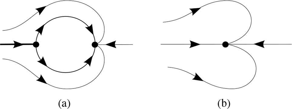
Clearly the origin corresponds to r = 0 which is invariant under the flow of system (4.12). On r = 0, taking into account that b > 1, we have two singular points which are θ = 0 and θ = π. Computing the eigenvalues of the Jacobian matrix at these points we get that (0,0) is a saddle if a < 1 and a stable node if a ⩾ 1 (when a = 1 this node is semi-hyperbolic). On the other hand the singular point (0,π) is a saddle if a > −1 and an unstable node if a ⩽ −1 (when a = −1 the node is semi-hyperbolic). To obtain the behavior of the origin of system (4.12) we identify θ = 0 and θ = 2π and r = 0 becomes a circle in the cylinder (r,θ) ∈ ℝ × 𝕊1. In this case the semi-cylinder r > 0 corresponds to the plane (x,y) of system (4.12) around the origin. So we are only interested in the separatrices (or dynamics) of system (4.12) in r > 0. Going back through the change of variables to obtain the local behavior at the origin, we need to shrink the circle to a point. This will be done for the different values of a. More precisely, when a ⩽ −1 we have the phase portrait in Figure 6(a) with r = 0 as a circle. Shrinking the circle to a point we conclude that the origin is an unstable node, see Figure 6(b). When a ∈ (−1,0)∪(0,1) we have the phase portrait in Figure 7(a) again with r = 0 as a circle. Going back through the change of variables we get that the origin is formed by two hyperbolic sectors, see Figure 7(b). Finally, when a ⩾ 1 we have the phase portrait in Figure 8(a) with r = 0 as a circle. Shrinking the circle to a point we conclude that the origin is a stable node, see Figure 8(b). This concludes the study of the finite singular points of system (4.10).
In the local chart U1 system (4.10) writes as
Since b > 1 system (4.13) has no infinite singular points. On the other hand system (4.10) in the local chart U2 becomes
Note that the origin of U2 is not a singular point. So the circle at infinity is a periodic solution.
Doing the rescaling of the time
Since the divergence of this system is
Global phase portraits of system (4.10) with b > 1 and a ≠ 0. (a): for |a| ⩾ 1, (b): a ∈ (−1,0) ∪ (0,1).
According to Lemma 2.1 for any trajectory γ not starting on the cone we have that ω(γ) and α(γ) are contained in the closure of the cone inside the Poincaré ball.
Assume now that 0 < b < 1. Again the cone x2 − y2 + (1 − b)z2/b = 0 is an invariant algebraic surface. System (1.1) restricted to this cone becomes either
Note that system (4.16) is the same as system (4.15) with a reparameterization of the time t ↦ −t and the parameter a interchanged by −a. So the behavior is the same with the stability interchanged and the values of a also changed to −a. Hence, we will study only system (4.15). However, the study of system (4.15) can be done in an analogous way to system (4.10), obtaining the phase portraits of Figure 9. Again, according to Lemma 2.1 for any trajectory γ not starting on the cone we have that ω(γ) and α(γ) are contained in the closure of the cone inside the Poincaré ball.
Acknowledgements
The first author is supported by the Ministerio de Economía, Industria y Competitividad - Agencia Estatal de Investigación grant MTM2016-77278-P (FEDER), the Agència de Gestió d’Ajuts Universitaris i de Recerca grant 2017 SGR 1617, and the European project Dynamics- H2020-MSCA-RISE-2017-777911. The second author is supported by CONICYT PCHA / Post-doctorado en el extranjero Becas Chile / 2018 - 74190062. The third author is partially supported by FCT/Portugal through UID/MAT/04459/2013.
References
Cite this article
TY  - JOUR
AU  - Jaume Llibre
AU  - Y. Paulina Martínez
AU  - Claudia Valls
PY  - 2020
DA  - 2020/05/04
TI  - On the global dynamics of a three-dimensional forced-damped differential system
JO  - Journal of Nonlinear Mathematical Physics
SP  - 414
EP  - 428
VL  - 27
IS  - 3
SN  - 1776-0852
UR  - https://doi.org/10.1080/14029251.2020.1757232
DO  - 10.1080/14029251.2020.1757232
ID  - Llibre2020
ER  -