Journal of Nonlinear Mathematical Physics

Volume 28, Issue 1, March 2021, Pages 38 - 52

Inverse Scattering Transformation for the Fokas–Lenells Equation with Nonzero Boundary Conditions

Authors
Yi Zhao, Engui Fan*
School of Mathematical Sciences, Fudan University, Shanghai 200433, P. R. China
*Corresponding author. Email: faneg@fudan.edu.cn
Corresponding Author
Engui Fan
Received 12 February 2020, Accepted 3 March 2020, Available Online 10 December 2020.
DOI
10.2991/jnmp.k.200922.003How to use a DOI?
Keywords
Fokas–Lenells equation; nonzero boundary conditions; inverse scattering transformation; Riemann–Hilbert problem; N-soliton solution
Abstract

In this article, we focus on the inverse scattering transformation for the Fokas–Lenells (FL) equation with nonzero boundary conditions via the Riemann–Hilbert (RH) approach. Based on the Lax pair of the FL equation, the analyticity, symmetry and asymptotic behavior of the Jost solutions and scattering matrix are discussed in detail. With these results, we further present a generalized RH problem, from which a reconstruction formula between the solution of the FL equation and the Riemann–Hilbert problem is obtained. The N-soliton solutions of the FL equation is obtained by solving the RH problem.

Copyright
© 2020 The Authors. Published by Atlantis Press B.V.
Open Access
This is an open access article distributed under the CC BY-NC 4.0 license (http://creativecommons.org/licenses/by-nc/4.0/).

1. INTRODUCTION

The Nonlinear Schrödinger (NLS) equation

iut+uxx-2ν|q|2q=0 (1.1)
with ν = ±1 is a significant mathematical and physical model for the optical fibers, deep water waves and plasma physics [3]. The NLS equation is a completely integrable system which admits Lax pair and bi-Hamiltonian formulation [21,22].

In the late 70s, standard bi-Hamiltonian formulation was used to obtain an integrable generalization of a given equation [7]. For instance, the Camassa–Holm equation is derived from the KdV equation via the bi-Hamiltonian structure [6], and the same mathematical trick can be applied to the NLS equation yields Fokas–Lenells (FL) equation [8]

iut-νutx+γuxx+σ|u|2(u+iνux)=0,σ=±1. (1.2)

If let α = γ/ν > 0 and β=1ν and

uβαeiβxu,σ-σ,
then equation (1.2) can be converted into
utx+αβ2u-2iαβux-αuxx+σiαβ2|u|2ux=0, (1.3)
where α, β > 0. In this paper, we consider the focusing case with σ = −1.

In recent years, much work has been done on the FL equation (1.3). For example, Lax pair for FL equation was obtained via the bi-­Hamiltonian structure by Fokas and Lenells [8]. They further considered the initial-boundary problem for the FL equation (1.3) on the half-line by using the Fokas unified method [9]. The dressing method is applied to obtain an explicit formula for bright-soliton and dark soliton solutions for Eq. (1.3) [11,15]. The bilinear method was used to obtain bright and dark soliton solution are obtained [12,13]. The Darboux transformation is used to obtain rogue waves of the FL equation [10,19]. The Deift–Zhou nonlinear steepest decedent method was used to analyze long-time asymptotic behavior for FL equation with decaying initial value [18]. Riemann–Hilbert (RH) approach was adopted to construct explicit soliton solutions under zero boundary conditions [1]. As far as we know, the soliton solutions for the FL equation (1.3) with Nonzero Boundary Conditions (NZBCs) have not been reported. In this paper, we apply RH approach to study the inverse transformation of the FL equation (1.3) with the following NZBCs

u(x,t)q±e-iβx+2iαβt,x±, (1.4)
where |q±|=2β and assume that u(x, t) − q±L1(R±); with respect to x for all t ≥ 0. In next section, we will see that this kind of NZBCs (1.4) avoids the discussion on a multi-valued function as the case of the NLS equation [3].

The inverse scattering transform is an important method to study important nonlinear wave equations with Lax pair such as the NLS equation, the modified KdV equation, Sine-Gordan equation [5,14]. As an improved version of inverse scattering transform, the RH method has been widely adopted to solve nonlinear integrable systems [2,4,16,17,20,23].

The paper is organized as follows. In Section 2, by introducing appropriate transformations, we change the asymptotic boundary conditions (1.4) into constant boundary conditions. Furthermore, we analyze the analyticity, symmetry and asymptotic behavior of eigenfunctions and scattering matrix associated with the Lax pair. In Section 3, a generalized RH problem for the FL equation is constructed, and the distribution of discrete spectrum and residue conditions associated with RH problem are discussed. Based on these results, we reconstruct the potential function from the solution of the RH problem. In Section 4, we give the N-soliton solutions via solving RH problem under reflectionless case.

2. THE DIRECT SCATTERING WITH NZBCS

2.1. Jost Solutions

It is well-known that the FL equation (1.3) admits a Lax pair

ψx+ik2σ3ψ=kUxψ,ψt+iη2σ3ψ=[αkUx+iαβ22σ3(1kU-U2)]ψ, (2.1)
where
U=(0uv0),σ3=(100-1),η=α(k-β2k),v=-u*.

In order to invert the nonzero boundary conditions into the constant boundary conditions, we introduce a transformation for eigenfunctions and potentials.

Theorem 2.1.

By transformation

u=qe-iβx+2iαβt,ψ=e(-12iβx+iαβt)σ3φ, (2.2)
the FL equation (1.3) becomes
qtx-iβqt+2iαβqx-αqxx+(2αβ2-αβ3|q|2)q-iαβ2|q|2qx=0 (2.3)
with corresponding boundary conditions
qq±,x±. (2.4)

And Eq. (2.3) is the compatibility condition of the Lax pair

φx=Xφ,φt=Tφ, (2.5)
where
X=-ik2σ3+12iβσ3-iβkσ3Q+kQx,T=-iη2σ3-12iαβ2σ3Q2-12iαβ2q02σ3-iαβkσ3Q+αkQx+iαβ22kσ3Q,
with Q=(0q-q*0).

Proof. Suppose the transformation is

u=qeAix+Bit,ψ=e(iCx+iDt)σ3φ.

Substituting it into (1.3) yields

qxt+Aiqt+i(B-2αβ-2αA)qx+(2αβA+αβ2+αA2-AB)q-αqxx+Aαβ2|q|2q-iαβ2|q|2qx=0. (2.6)

And the Lax pair becomes

φx=e[i(A2-C)x+i(B2-D)t]σ^3(-ik2-iCk(Aiq+qx)k(Aiq*-qx*)ik2+iC)φ,φt=e[i(A2-C)x+i(B2-D)t]σ^3(-iη2+12iαβ2|q|2-iDαk(Aiq+qx)+iαβ22kq-αk(-Aiq*+qx*)+iαβ22kq*iη2-12iαβ2|q|2+iD)φ. (2.7)

Take A = 2C and B = 2D in the above equation and consider the limit as x → ±∞, one gets

X±=(-ik2-A2ikAiq±kAiq±*ik2+A2i),T±=(-iη2+iαβ-iDαkiAq±+iαβ22kq±αkiAq±*+iαβ22kq±*iη2-iαβ+iD).

These two matrices are proportional if

A=-β,B=2αβ.

Moreover, T± and X± are proportional

T±=αηkX±.
which implies that their eigenvalues are proportional and they share the same eigenvector matrices.

To diagonalize the matrices X± and T± and further obtain the Jost solutions, we need to get the eigenvalues and eigenvector matrices of them. Direct calculation shows that the eigenvalues of the matrices X± are ±ikαλ ; and the eigenvalues of the matrices T± are ±iηλ, where

λ=α(k+β2k),
and the corresponding eigenvector matrices are
Y±(k)=I-β2kQ±,detY±(k)=1+β2k2γ(k),
with Q±=(0q±-q±*0).

With the above results, the matrices can be diagonalized as:

X±=Y±(-ikλσ3α)Y±-1,T±=Y±(-iηλσ3)Y±-1. (2.8)

Thus, the asymptotic Lax pair

φ˜x=X±φ˜,φ˜t=T±φ˜ (2.9)
can be written as
(Y±-1φ˜)x=-ikλσ3α(Y±-1φ˜),(Y±-1φ˜)t=-iησ3(Y±-1φ˜),
which has a solution
φ˜=Y±(k)e-iθ(x,t,k)σ3. (2.10)

Therefore, the asymptotic of the eigenfunctions φ± are

φ±Y±(k)e-iθ(x,t,k)σ3,x±, (2.11)
where
θ(x,t,k)=kλxα+ληt.

Define the Jost solutions as

J±(x,t,k)=φ±(x,t,k)eiθσ3, (2.12)
then the Lax pair (2.5) is changed to
J±,x-ikλαJ±σ3=XJ±,J±,t-iληJ±σ3=TJ±, (2.13)
and
J±Y±(k),x±. (2.14)

2.2. Scattering Matrix

The functions φ± are both fundamental matrix solutions of the Lax pair (2.5), thus there exists a matrix S(k) that only depends on k, such that

φ+(x,t,k)=φ-(x,t,k)S(k), (2.15)
where S(k) is called scattering matrix. Columnwise, Eq. (2.15) reads
φ+,1=s11φ-,1+s21φ-,2,φ+,2=s12φ-,1+s22φ-,2. (2.16)

Since tr(X) = tr(T) = 0, according to the Abel’s formula, we have

(detφ±)x=(detφ±)t=0,
which implies
detφ±=limx±detφ±=γ(k),
then the scattering coefficients can be expressed as Wronskians of columns φ± in the following way
s11(k)=Wr(φ+,1,φ-,2)γ(k),s12(k)=Wr(φ+,2,φ-,2)γ(k),s21(k)=Wr(φ-,1,φ+,1)γ(k),s22(k)=Wr(φ-,1,φ+,2)γ(k). (2.17)

2.3. Asymptotic Analysis

To properly construct the Riemann–Hilbert problem, we need to consider the asymptotic behavior of eigenfunctions and scattering matrix as k → ∞ and k → 0.

2.3.1. Asymptotic as k → ∞

Consider a solution of (2.13) of the form

J±=J±(0)+J±(1)k+J±(2)k2+,
then substituting the above expansion into (2.13) and comparing the coefficients of the same order of k, we get the comparison results:

x-part:

O(k0):J±,x(0)+i[σ3,J±(2)]=iβσ3J±(0)-iβσ3QJ±(1)+QxJ±(1), (2.18)
O(k2):J±(0)σ3=σ3J±(0). (2.19)
t-part:
O(k):[σ3,J±(1)]=-βσ3QJ±(0)-iQxJ±(0), (2.20)

O(k0):J±,t(0)+iα[σ3,J±(2)]=iαβσ3J±(0)-12iαβ2Q2σ3J±(0)-12iαβ2q02σ3J±(0)-iαβσ3QJ±(1)+αQxJ±(1). (2.21)

Based on these results, we derive that J±(0) is diagonal and satisfies

J±,x(0)=iν1σ3J±(0), (2.22)
J±,t(0)=iν2σ3J±(0), (2.23)
where
ν1(x,t)=β+12β2qr-12iβqrx+12iβqxr+12qxrx,ν2(x,t)=αβ-12αβ2q02+12iαβ(qxr-qrx)+12αqxrx.

Note that the FL equation (2.3) admits the conservation law

(qxrx-iβqrx+iβqxr+β2qr)t=(αqxrx+iαβ(qxr-qrx))x,
thus Eqs. (2.22) and (2.23) are consistent and are both satisfied if we define
J±(0)=eiνσ3,ν=-x(β+12β2qr-12iβqrx+12iβqxr+12qxrx)dx. (2.24)

Therefore, we obtain the limit of the Jost solutions as k → ∞:

J±J±(0),k. (2.25)

Define

J±=J±(0)μ±, (2.26)
then we have
μ±I,k. (2.27)

In addition, the asymptotic property of φ± follows:

φ±ei(ν-θ)σ3,k.

Consider the wronskians expression of the scattering coefficients (2.17), we find that

s11(k)1,s22(k)1,k. (2.28)

2.3.2. Asymptotic as k → 0

We first assume that J± admit a Lorrent expansion

J±=n=-n=knD±(n).

Substituting into (2.13) and comparing the coefficients of the same order of k gives that D±(n)=0,n=-2,-3, . Thus we expend solution of (2.13) of the form

J±=D±(-1)k+D±(0)+D±(1)k+,
then we obtain the comparison results:

x-part:

O(k-1):D±,x(-1)-12iβD±(-1)σ3=12iβσ3D±-1, (2.29)

t-part:

O(k-3):D±-1σ3=-σ3D±-1. (2.30)

It is easy to check that

D±,x(-1)=0, (2.31)
which implies D±(-1) is a constant independent on x. This implies that the following limit
limk0kJ±=D±(-1) (2.32)
is uniformly convergent for xR. While the following limit
limx±kJ±=kI-β2Q± (2.33)
exists for every fixed kC. Thus the following limit is commutative, and using (2.32) and (2.33) yields
D±(-1)=limx±limk0kJ±=limk0limx±kJ±=-β2Q±,
which leads to
J±=-βQ±2k+O(1),k0. (2.34)

The asymptotics of functions φ± and μ± can be obtained by transformations (2.12) and (2.26). Consider the wronskian expressions of scattering coefficients and note the boundary conditions, we find that

s11=Wr(J+,1e-iθ,J-,2eiθ)=q-q++O(1),k0,s22=Wr(J-,1e-iθ,J+,2eiθ)=q-*q+*+O(1),k0.

2.4. Analyticity

Noticing that

Im(kλα)=4RekImk,
we define two domains and their boundary
D+={k|RekImk>0}={k|argk(0,π2)(π,32π)},D-={k|RekImk<0}={k|argk(π2,π)(32π,2π)},Σ={k|RekImk=0}=RiR.
which are shown in Figure 1.

Figure 1

The jump contour in the complex k-plane.

Under the transformation (2.26), we write the Lax pair as

μ±,x-ikλα[μ±,σ3]=X^μ±,μ±,t-iλη[μ±,σ3]=T^μ±, (2.35)
where
X^=e-iνσ^3(X+ikλσ3α-iν1σ3),T^=e-iνσ^3(T+iλησ3-iν2σ3).

We rewrite the Eq. (2.35) into a full differential form

d(eiθσ^3μ±)=eiθσ^3(X^dx+T^dt)μ±, (2.36)
which implies μ± can be formally integrated to obtain the integral equations for the eigenfunctions:
μ-=μ-0+-xe-ikλα(x-y)σ^3X^(y,t,k)μ-(y,t,k)dy, (2.37)

μ+=μ+0-x+e-ikλα(x-y)σ^3X^(y,t,k)μ+(y,t,k)dy, (2.38)

where

μ-0=Y-,μ+0=e-i-+ν1(x')dx'σ3Y+.

By using a similar way to Appendix A in Biondini and Kovačič [1], under mild integrability conditions on the potential, the eigenfunctions (2.37) and (2.38) can be analytically extended in the complex k-plane into the following regions:

μ-,1,μ+,2:D+,μ+,1,μ-,2:D-, (2.39)
where μ± = (μ±,1, μ±,2), the subscript 1, 2 denote the first and second column of μ±.

Apparently, the functions φ± and μ± share the same analyticity, hence from the wronskians expression of the scattering coefficients, we know that s11 is analytic in D, and s22 is analytic in D+.

2.5. Symmetry

To investigate the discrete spectrum and residue conditions in the Riemann–Hilbert problem, one needs to analyze the symmetric property for the solutions φ± and the scattering matrix S(k).

Theorem 2.2.

The Jost eigenfunctions satisfy the following symmetric relations

σφ±*(k*)σ=-φ±(k), (2.40)
σ1φ±*(-k*)σ1=φ±(k), (2.41)
and the scattering matrix satisfies
-σS(k)σ=S*(k*), (2.42)
σ1S*(-k*)σ1=S(k). (2.43)
where
σ=(01-10),σ1=(0110).

Proof. We only prove (2.40) and (2.42), (2.41) and (2.43) can be shown in a similar way. The functions φ± are the solutions of the spectral problem

φ±,x(k)=X(k)φ±(k). (2.44)

Conjugating and multiplying left by σ on both sides of the equation gives

(σφ±*(k*)σ)x=σX*(k*)φ±*(k*)σ.

Note that σX*(k*) = X(k)σ, hence σφ±*(k*)σ is also a solution of (2.44). By using relations σY±*(k*)=Y±(k)σ and σeiθσ3σ=-e-iθσ3 , we obtain

σφ±*(k*)σ-Y±(k)e-iθσ3,x±, (2.45)
which leads to (2.40).

For the scattering matrix, conjugating on the both sides of Eq. (2.15) leads to

φ+*(k*)=φ-*(k*)S*(k*),
substituting (2.40) into the above formula yields
φ+(k)=-φ-(k)σS*(k*)σ,
comparing with (2.15) gives
S*(k*)=-σS(k)σ.

Elementwise, Eqs. (2.40)(2.43) read as

s11*(k*)=s22(k),s21*(k*)=-s12(k),s11*(-k*)=s22(k),s21*(-k*)=s12(k). (2.46)
φ±,1(k)=σφ±,2*(k*),φ±,2(k)=-σφ±,1*(k*),φ±,1(k)=σ1φ±,2*(-k*),φ±,2(k)=σ1φ±,1*(-k*), (2.47)
which implies
φ±,2(k)=-σ3φ±,2(-k),φ±,1(k)=σ3φ±,1(-k), (2.48)
note the relation (2.12) and (2.26), there exists
φ±=eiνσ3μ±e-iθσ3, (2.49)
thus for the eigenfunctions μ±, we derive
μ±,2(k)=-σ3μ±,2(-k),μ±,1(k)=σμ±,1(-k). (2.50)

3. THE INVERSE SCATTERING WITH NZBCS

3.1. Generalized Riemann–Hilbert Problem

We define the two matrices

M+=(μ-,1,μ+,2s22),kD+,M-=(μ+,1s11,μ-,2),kD-,
which are analytical in D+, D respectively, and admit asymptotic
M±=I+O(1/k),k,M±=1ke-iνσ3Q˜-+O(1),k0, (3.1)
where Q˜-=(0-1q-*1q-0) .

By using (2.49) and (3.1), we rewrite (2.16) and get a generalized Riemann–Hilbert problem

M(x,t,k)ismeromorphicinC\Σ, (3.2)

M+(x,t,k)=M-(x,t,k)(I-G(x,t,k)),kΣ, (3.3)
M(x,t,k)satisfiesresidueconditionsatzeros{k:s11(k)=s22(k)=0}, (3.4)
M±=I+O(1/k),k, (3.5)
M±=1ke-iνσ3Q˜±+O(1),k0, (3.6)

where the jump matrix

G=(0-e-2iθρ˜(k)e2iθρ(k)ρ(k)ρ˜(k)),ρ(k)=s21s11,ρ˜(k)=s12s22.
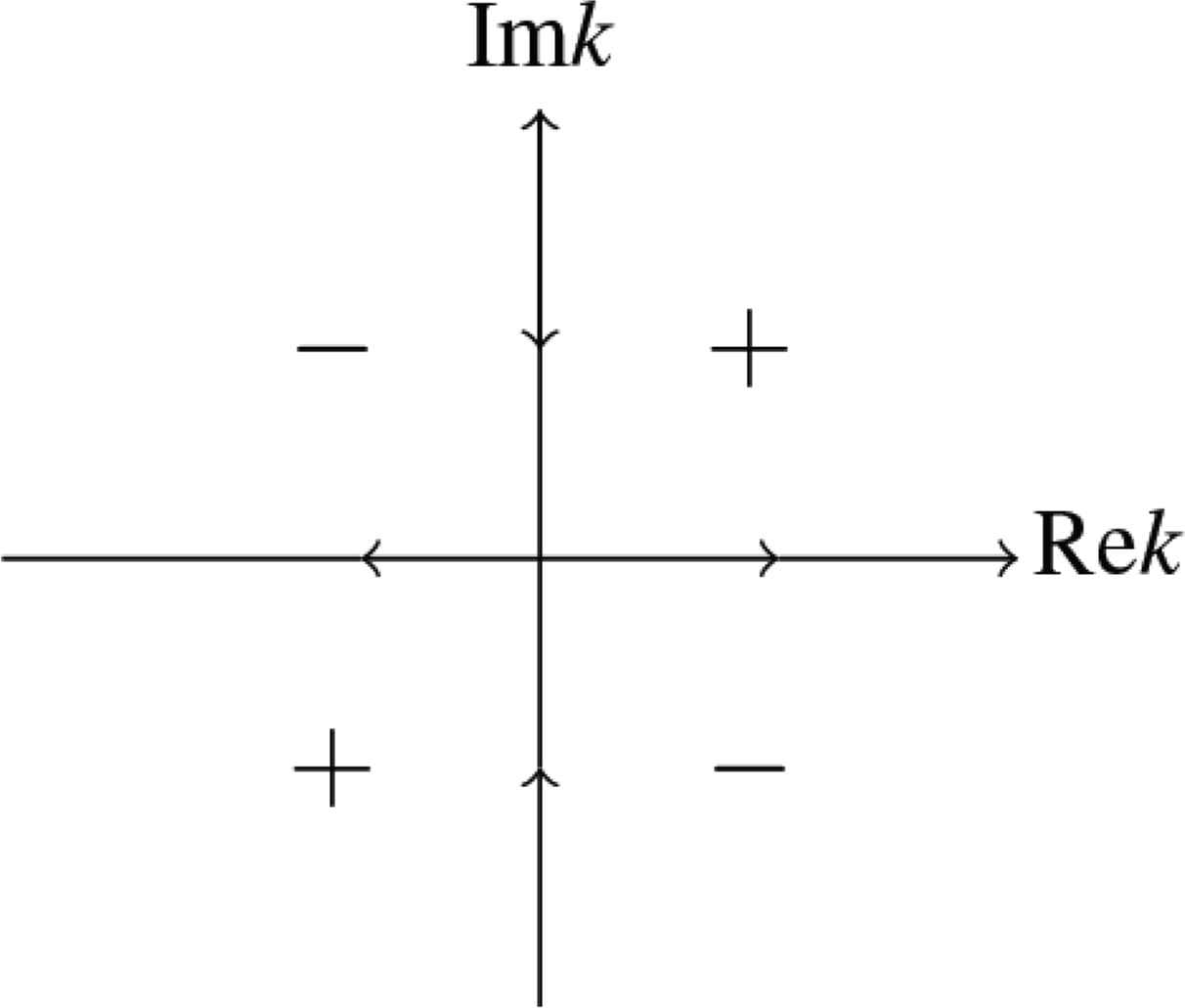
and Σ = R ∪ iR denotes the jump contour in Figure 1.

3.2. Discrete Spectrum and Residue Conditions

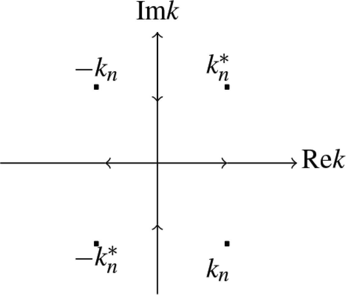
Suppose that s11(k) has N simple zeroes in D+ ∩{Im k < 0} denoted by kn, n = 1, 2, ..., N. Owing to the symmetries in (2.46), there exists

s11(kn)=0s22(-kn*)=0s22(kn*)=0s11(-kn)=0,
thus the discrete spectrum is the set
{±kn,±kn*}, (3.7)
which distribute in the k-plane as shown in Figure 2.

Figure 2

Discrete spectrum.

Next we derive the residue conditions will be needed for the RH problem. If s11(k) = 0 at k = kn the eigenfunctions φ+,1 and φ−,2 at k = kn must be proportional

φ+,1(kn)=bnφ-,2(kn), (3.8)
where bn is an arbitrary constant independent on x, t. Under the transformation (2.49), there exists linear relation for μ±
μ+,1(kn)=bne2iθ(kn)μ-,2(kn). (3.9)

Thus we get

Resk=kn[μ+,1s11]=μ+,1(kn)s11'(kn)=Cne2iθ(kn)μ-,2(kn), (3.10)
where Cn=bns11'(kn) . As for k = −kn, substituting (2.48) into (3.8) leads to
φ+,1(-kn)=-bnφ-,2(-kn), (3.11)
then applying the relation (2.49) yields
μ+,1(-kn)=-bne2iθ(kn)μ-,2(-kn), (3.12)
thus we obtain
Resk=-kn[μ+,1s11]=μ+,1(-kn)s11'(-kn)=-Cne2iθ(kn)σ3μ-,2(kn). (3.13)

Similarly, the residue conditions at k=±kn* are

Resk=kn*[μ+,2s22]=μ+,2(kn*)s22'(kn*)=C˜ne-2iθ(kn*)μ-,1(kn*), (3.14)

Resk=-kn*[μ+,2s22]=μ+,2(-kn*)s22'(-kn*)=C˜ne-2iθ(kn*)σ3μ-,1(kn*), (3.15)

where C˜n=-Cn* .

Recall the definition of M±, there follows

Resk=kn*M+=(0,C˜ne-2iθ(kn*)μ-,1(kn*)),Resk=-kn*M+=(0,C˜ne-2iθ(kn*)σ3μ-,1(kn*)),Resk=knM-=(Cne2iθ(kn)μ-,2(kn),0),Resk=-knM-=(-Cne2iθ(kn)σ3μ-,2(kn),0). (3.16)

3.3. Reconstruction Formula for the Potential

To solve the Riemann–Hilbert problem (3.3), one needs to regularize it by subtracting out the asymptotic behaviour and the pole contribution. Hence, we rewrite Eq. (3.3) as

M+-I-1ke-iνσ3Q˜--n=1NResk=kn*M+k-kn*-n=1NResk=knM-k-kn-n=1NResk=-kn*M+k+kn*-n=1NResk=-knM-k+kn=M--I-1ke-iνσ3Q˜--n=1NResk=kn*M+k-kn*-n=1NResk=knM-k-kn-n=1NResk=-kn*M+k+kn*-n=1NResk=-knM-k+kn-M-G, (3.17)
where Q˜-=(0-1q-*1q-0) . Then the Plemelj’s formula shows
M(x,t,k)=I+1ke-iνσ3Q˜-+n=1NResk=kn*M+k-kn*+n=1NResk=knM-k-kn+n=1NResk=-kn*M+k+kn*+n=1NResk=-knM-k+kn+12πiΣM-G(x,t,ξ)ξ-kdξ, (3.18)
and the (1, 2)-element of M is
M12=1k{e-iνσ3Q˜-+n=1N(Resk=kn*M++Resk=-kn*M+)-12πiΣM-G(x,t,ξ)ξ-kdξ}12+O(1/k2). (3.19)

Comparing the (1, 2)-element on the both sides of Eq. (2.20) yields

qx-iβq=2ieiνJ±,12(1). (3.20)

Recall the transformation (2.2), we know

uxeiτ(x,t)=qx-iβq,
where τ(x,t)=βx+αβ2q02t. Thus we can write (3.20) as
ux=2ieiν-iτlimk(kJ±)12=2ie2iν-iτlimk(kμ±)12=2ie2iν-iτ(M1-)12, (3.21)
where
M-=M0-+M1-k+.

Substituting (3.19) and (3.16) into (3.21), we obtain the reconstruction formula for potential

ux=2ie2iν-iτ{e-iνq-*+2n=1NC˜ne-2iθ(kn*)μ-,1,1(kn*)-12πiΣ(M-G)12(ξ)dξ}. (3.22)

4. REFLECTIONLESS POTENTIALS

Now we consider the potential u(x, t) for which the reflection coefficient ρ(k) vanishes identically, that is, G = 0. In this case, Eq. (3.22) reads as

ux=2ie-iτ(n2e2iνC˜ne-2iθ(kn*)μ-,1,1(kn*)-eiνq-*). (4.1)

To obtain the expression of the term μ-,1,1(kn*) , we consider the first and second column of (3.18) respectively under reflectionless case:

μ-,2(kn)=(-e-iνknq-*1)+j=1NC˜je-2iθ(kj*)kn-kj*μ-,1(kj*)+j=1NC˜je-2iθ(kj*)kn+kj*σ3μ-,1(kj*),μ-,1(kn*)=(1eiνkn*q-)+j=1NCje2iθ(kj)kn*-kjμ-,2(kj)-j=1NCje2iθ(kj)kn*+kjσ3μ-,2(kj), (4.2)
which can be further written as
μ-,2(kn)=(-e-iνknq-*1)+2j=1NC˜je-2iθ(kj*)kn2-(kj*)2K1μ-,1(kj*),μ-,1(kn*)=(1eiνkn*q-)+2j=1NCje2iθ(kj)(kn*)2-kj2K2μ-,2(kj), (4.3)
where
K1=(kn00kj*),K2=(kj00kn*).

Define

cj(x,t,k)=Cj(k*)2-kj2e2iθ(x,t,kj),
whose conjugate gives
cj*(k)=-C˜jk2-(kj*)2e-2iθ(kj*).

Then (4.3) reduces to

μ-,1,1(kn*)=1+2j=1Nkjcj(kn)μ-,1,2(kj), (4.4)

μ-,1,2(kj)=-e-iνkjq-*-2m=1Nkjcm*(kj)μ-,1,1(km*), (4.5)

substituting (4.5) into (4.4) yields

μ-,1,1(kn*)=1-2e-iνq-*j=1Ncj(kn)-4j=1Nm=1Nkj2cj(kn)cm*(kj)μ-,1,1(km*),n=1,2,,N. (4.6)

Introducing notations

X=(X1,X2,,XN)t,A=(An,m),B=(B1,B2,,BN)t
with components being
Xn=μ-,1,1(kn*),Anm=j=1N4kj2cj(kn)cm*(kj),Bn=1-2e-iνq-*j=1Ncj(kn),
then the system (4.6) can be written as matrix form
HX=B, (4.7)
where
H=I+A=(H1,H2,,HN).

By standard Crammer rule, the system (4.7) is the solution of

μ-,1,1(kn*)=Xn=detHnextdetH, (4.8)
where
Hnext=(H1,,Hn-1,B,,HN).

Note that

uxvx=qxrx+iβqxr-iβqrx+β2qr,
then Eq. (2.24) reduces to
ν=-x(β+12uxvx)(x',t)dx', (4.9)

Therefore, we obtain a compact solution:

ux=2ie-iτ(x,t)+iν(detHaugdetHeiν-1q-*), (4.10)
where the augmented (N + 1) × (N + 1) matrix Haug is
Haug=(0YtBH),Y=(Y1,,YN)t,
and Yn=2C˜ne-2iθ(kn*)=-2Cn*e-2iθ(kn*) .

5. TRACE FORMULA AND THETA CONDITION

Define

β-=s11(k)n=1Nk2-(kn*)2k2-kn2,β+=s22(k)n=1Nk2-kn2k2-(kn*)2, (5.1)
we see that they are analytic and no-zeros in D and D+, respectively. Moreover, β+ β = s11(k)s22(k). Note that det S(k) = s11s22s21s12 = 1, this implies
1s11s22=1-ρ(k)ρ˜(k)=1+ρ(k)ρ*(k*),
thus
β+β-=s11s22=11+ρ(k)ρ*(k*),kΣ.

Taking logarithms leads to

logβ+-(-logβ-)=-log[1+ρ(k)ρ(k*)],kΣ,
then Applying Plemelj formula, we have
logβ±=12πiΣlog[1+ρ(s)ρ*(s*)]s-kds,kD±. (5.2)

Substituting into (5.1), we obtain the trace formula

s11(k)=exp[12πiΣlog[1+ρ(s)ρ*(s*)]s-kds]n=1Nk2-kn2k2-(kn*)2,kD-,s22(k)=exp[-12πiΣlog[1+ρ(s)ρ*(s*)]s-kds]n=1Nk2-(kn*)2k2-kn2,kD+. (5.3)

Under reflectionless condition, they reduce to

s11(k)=n=1Nk2-kn2k2-(kn*)2,kD-;s22(k)=n=1Nk2-(kn*)2k2-kn2,kD+. (5.4)

Taking limit as k → 0 for (5.4) leads to

q-βq+=exp[-i2πΣlog[1+ρ(s)ρ*(s*)]sds]exp[4in=1Narg(kn)],kD-, (5.5)
note that β is a positive constant, then we obtain the theta condition
arg(q-q+)=-12πΣlog[1+ρ(s)ρ*(s*)]sds+4n=1Narg(kn). (5.6)
under reflectionless condition, we have
arg(q-q+)=4n=1Narg(kn). (5.7)

6. ONE-SOLITON SOLUTION

As an application of the formula (4.10) of N-soliton solution, we construct one-soliton solution for the FL equation, which corresponds to N = 1. Then Eq. (4.10) becomes

ux=2ie-iτ+iν(-2C1*e-2iθ(k1*)eiν1+4k12|c1(k1)|2+(4+4β)C1*e-2iθ(k1*)c1(k1)q-*(1+4k12|c1(k1)|2)-1q-*), (6.1)
where k1 is an eigenvalue, C1 is an arbitrary constant and
θ(k1)=k1λ1αx+λ1η1t,λ1=α(k1+β2k1),η1=α(k1-β2k1),c1(k1)=C1(k1*)2-k12e2iθ(k1). (6.2)

CONFLICTS OF INTEREST

The authors declare they have no conflicts of interest.

ACKNOWLEDGMENT

This work is supported by the National Science Foundation of China (Grant No. 11671095, 51879045).

REFERENCES

[15]VE Vekslerchik, Lattice representation and dark solitons of the Fokas–Lenells equation, Nonlinearity, Vol. 24, 2011, pp. 1165.
[16]L Wen and E Fan, The Sasa-Satsuma equation with non-vanishing boundary conditions. arXiv: 1911.11944.
[20]Y Yang and E Fan, Riemann-Hilbert approach to the modified nonlinear Schrödinger equation with non-vanishing asymptotic boundary conditions. arXiv: 1910.07720.
[21]VE Zakharov and AS Fokas, Important Developments in Soliton Theory, Springer Science & Business Media, 2012.
[22]VE Zakharov and AB Shabat, Exact theory of two-dimensional self-focusing and one-dimensional self-modulation of waves in nonlinear media, J. Exp. Theor. Phys., Vol. 34, 1972, pp. 62-69.
Journal
Journal of Nonlinear Mathematical Physics
Volume-Issue
28 - 1
Pages
38 - 52
Publication Date
2020/12/10
ISSN (Online)
1776-0852
ISSN (Print)
1402-9251
DOI
10.2991/jnmp.k.200922.003How to use a DOI?
Copyright
© 2020 The Authors. Published by Atlantis Press B.V.
Open Access
This is an open access article distributed under the CC BY-NC 4.0 license (http://creativecommons.org/licenses/by-nc/4.0/).

Cite this article

TY  - JOUR
AU  - Yi Zhao
AU  - Engui Fan
PY  - 2020
DA  - 2020/12/10
TI  - Inverse Scattering Transformation for the Fokas–Lenells Equation with Nonzero Boundary Conditions
JO  - Journal of Nonlinear Mathematical Physics
SP  - 38
EP  - 52
VL  - 28
IS  - 1
SN  - 1776-0852
UR  - https://doi.org/10.2991/jnmp.k.200922.003
DO  - 10.2991/jnmp.k.200922.003
ID  - Zhao2020
ER  -