
Classifying image analysis techniques from their output
Facultad de Ciencias Matemáticas, Complutense University, Plaza de las Ciencias 3, Madrid, 28040, Spain.
Facultad de Ciencias Matemáticas, Complutense University, Plaza de las Ciencias 3, Madrid, 28040, Spain.
Facultad de Estudios Estadísticos, Complutense University, Av. Puerta de Hierro s/n, Madrid, 28040, Spain.
Instituto de Geociencias IGEO (CSIC-UCM), Plaza de las Ciencias 3, Madrid, 28040, Spain.
- DOI
- 10.1080/18756891.2016.1180819How to use a DOI?
- Keywords
- Image segmentation; image classification; edge detection; fuzzy sets; machine learning; graphs
- Abstract
In this paper we discuss some main image processing techniques in order to propose a classification based upon the output these methods provide. Because despite a particular image analysis technique can be supervised or unsupervised, and can allow or not the existence of fuzzy information at some stage, each technique has been usually designed to focus on a specific objective, and their outputs are in fact different according to each objective. Thus, they are in fact different methods. But due to the essential relationship between them they are quite often confused. In particular, this paper pursues a clarification of the differences between image segmentation and edge detection, among other image processing techniques.
- Copyright
- © 2016. the authors. Co-published by Atlantis Press and Taylor & Francis
- Open Access
- This is an open access article under the CC BY-NC license (http://creativecommons.org/licences/by-nc/4.0/).
1. Introduction
Image analysis or image processing has become a scientific hot topic during the last decades, particularly because of the increasing amount of relevant information being stored in this format. Image analysis has a wide range of applications in different areas as remote sensing, image and data storage for transmission in business applications, medical imaging, acoustic imaging and security, among many other fields. Digital image processing techniques are being increasingly demanded through all areas of science and industry.
Many different techniques are considered “image processing” or “image analysis” techniques. Usually, each technique is appropriate for some a small range of tasks or for a specific problem.
For example, machine learning algorithms used in image analysis help in finding solutions to many problems in speech recognition 1, robotics 2 and vision 3. Computer vision uses image processing algorithms to extract significant information automatically from images. A number of algorithms are available to analyze images and recognize objects in them, and depending on the delivered output and the manner in which the images were encoded, specific learning methodologies are needed 4.
Another well-known example is image segmentation. Image segmentation methods try to simplify an image into something of easier analysis. Usually the image is transformed into segments or regions. These regions are supposed to be connected and represent a set of homogeneous pixels. Nevertheless, it is not clear when certain techniques should be considered as image segmentation methods, and such a situation also applies to other image processing techniques. It is quite common to classify two methods in the same group of techniques even if the output and the information they provide are very different. This is the case, for example, of edge detection methods 5, clustering image 6 and image thresholding algorithms 7, all of them classified as “image segmentation procedures” despite the obvious differences in their outputs.
There is a significant difference between image classification methods, edge detection methods, image segmentation methods and hierarchical image segmentation methods. Particularly, besides the strong relationship between them, all these methods address different problems, and produce different outputs. However, those different methods are not always clearly differentiated in the literature, and sometimes even confused. This paper poses a critical view on some of these techniques in order to show the conceptual differences between them. Depending on how a particular algorithm detects objects in an image and shows the output, the method might be understood as either performing classification, detection, segmentation or hierarchical segmentation.
Hence, the main objective of this paper is to present a classification of a set of widely used image processing algorithms, attending to the problems they face, the learning scheme they are based on, and the representational framework they utilize. Some new image analysis concepts and methods are also provided.
In order to understand the remainder paper, the following notation is adopted. The image we consider is being modeled as a two-dimensional function, where x and y are the coordinates in a plane, and f(x, y) represents each pixel by a fixed number of measurable attributes 8. Formally, an image can be defined as I = {f(x, y);x = 1,...,n and y = 1,...m} which can be represented computationally in:
- •
Binary ≡ f(x, y) ∈ {0, 1}.
- •
Gray ≡ f(x, y) ∈ {0,...,255}.
- •
RGB ≡ f(x, y) ∈ {0,...,255} 3.
A binary image is represented as a matrix allowing two possible values for each cell, two-tone colors (usually 0 refers to black and 1 to white). Similarly, a grey scale image may be defined as a two dimensional function f(x, y) where the amplitude of f at any pair of coordinates (x, y) refers to the intensity (gray level) of the image at that point. Instead, a color image is defined by a combination of individual 2D images. For instance, the RGB color system represents a color image in three components (red, green and blue). That is, it has an array of three matrices of equal size where the intensity of color of a pixel compound is represented by the three colors 8.
Figures 1, 2 and 3 show a binary image, a grayscale image and RGB image, respectively.

Binary image.

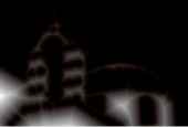
Gray level image.

RGB image 9.
The remainder of this paper is organized as follows: a review on image classification is presented in Section 2. Section 3 is devoted to fuzzy image classification. Some edge detection techniques are shown in Section 4, which is extended to fuzzy edge detection in Section 5. Image segmentation and some methods addressing this problem are analyzed in Section 6. Section 7 pays attention to hierarchical image segmentation. In Section 8 fuzzy image segmentation is addressed. Finally, some conclusions are shed.
2. Image classification
Classification techniques have been widely used in image processing to extract information from images by assigning each pixel to a class. Therefore, two types of outputs can be obtained at the end of an image classification procedure. The first kind of output is a thematic map where pixels are accompanied by a label for identification with a class. The second kind of output is a table summarizing the number of image pixels belonging to each class. Furthermore, both supervised and unsupervised learning schemes are applied for this image classification task 10. Next we provide an overview of these methods.
2.1. Supervised classification
Supervised classification is one of the most used techniques for image analysis, in which the supervisor provides information to the system about the categories present in each pattern in the training set.
Neural networks 11, genetic algorithms 12, support vector machines 13, bayesian networks 14, maximum likelihood classification 15 or minimum distance classification 16 are some techniques for supervised classification. Depending on certain factors such as data source, spatial resolution, available classification software, desired output type and others, it is more appropriate to use one of them to process a given image.
Supervised classification procedures are essential analytical tools for extracting quantitative information from images. According to Richards and Jia 4, the basic steps to implement these techniques are the following:
- •
Decide the classes to be identified in the image.
- •
Choose representative pixels of each class which will form the training data.
- •
Estimate the parameters of the algorithm classifier using the training data.
- •
Categorize all the remaining pixels in the image with the classifier in each of regions desired.
- •
Summarize the classification results in tables or display the segmented image.
- •
Evaluate the accuracy of the final model using a test data set.
A variety of classification techniques such as those mentioned above have been used in image analysis. In addition, some of those methods have been jointly used (e.g., neural networks 17,18, genetic algorithm with multilevel thresholds 19 or some variant of support vector machines 20).
In general, supervised classification provides good results if representative pixels of each class are chosen for the training data 4. Next, we pay attention to methods for unsupervised classification.
2.2. Unsupervised classification, clustering
Unsupervised classification techniques are intended to identify groups of individuals having common characteristics from the observation of several variables for each individual. In this sense, the main goal is to find regularities in the input data, because unlike supervised classification techniques, there is no supervisor to provide existing classes. The procedure tries to find groups of patterns, focussing in those that occur more frequently in the input data 21.
According to Nilsson 22, unsupervised classification consists of two stages to find patterns:
- •
Form a partition R of the set Ξ of unlabeled training patterns. The partition separates Ξ into mutually exclusive and exhaustive subsets R known as clusters.
- •
Design a classifier based on the labels assigned to the training patterns by the partition.
Clustering 23 is perhaps the most extended method of unsupervised classification for image processing, which obtains groups or clusters in the input image.
Particularly, cluster analysis looks for patterns in images, gathering pixels within natural groups that make sense in the context studied 21. The aim is that the proposed clustering has to be somehow optimal in the sense that observations in a cluster have to be similar, and in turn be dissimilar to those of other clusters. In this way, we try to maximize the homogeneity of objects within the clusters while the heterogeneity between aggregates is maximized. In principle, the number of groups to form and the groups themselves is unknown 24.
A standard cluster analysis creates groups that are as homogeneous as possible, and in turn the difference between the various groups is as large as possible. The analysis consist on the main following steps:
- •
First, we need to measure the similarity and dissimilarity between two separate objects (similarity measures the closeness of objects, so closer values suggest more homogeneity).
- •
Next, similarity and dissimilarity between clusters is measured so that the difference between groups become larger and thus group observations become as close as possible.
In this manner, the analysis can be divided into these two basic steps, and in both steps we can be use correlation measures or any distance 25 as similarity measure. Some similarity and dissimilarity measures for quantitative features are shown in 26.
Correlation measurements refer to the measurement of similarity between two objects in a symmetric matrix. If the objects tend to be more similar, the correlations are high. Conversely, if the objects tend to be more dissimilar, then the correlations are low. However, because these measures indicate the similarity by pattern matching between the features and do not observe the magnitudes of the observations, they are rarely used in cluster analysis.
Distance measurements represent the similarity and proximity between observations. Unlike correlation measurements, these similarity measures of distance or proximity are widely used in cluster analysis. Among the distance measures available, the most common are the Euclidean distance or distance metric, the standardized distance metric or the Malahanobis distance 26.
Let X(n × p) be a symmetric matrix with n observations of p variables. The similarity between the observations can be described by the matrix D(n × n):
Once a measure of similarity is calculated, we are able to proceed with the formation of clusters. A popular algorithm is k-means clustering 27. The algorithm was first proposed in 1957 by Lloyd 28 and published much later 29. K-means clustering algorithm classifies the pixels of the input image into multiple classes according to the distance from each other. The points are clustered around centroids μi, i = 1,...k obtained by minimizing the Euclidean distance. Let x1 and x2 be two pixels whose Euclidean distance between them is:
Thus, the sum of distances to k-center is minimized, and the objective is to minimize the maximum distance from every point to its nearest center 30.
Then, having selected the centroids, each observation is assigned to the most similar cluster based on the distance of the observation and the mean of the cluster. The average of the cluster is then recalculated, beginning an iterative process of centroid location depending on how observations are assigned to clusters; until the criterion function converges 31.
Clustering techniques have been used to perform unsupervised classification for image processing since 1969, when an algorithm finding boundaries in remote sensing data was proposed 32. Clustering implies grouping the pixels of an image in the multispectral space 4. Therefore, clustering seeks to identify a finite set of categories and clusters to classify the pixels, having previously defined a criteria of similarity between them. There are a number of available algorithms 33.
The resulting image of the k-means clustering algorithm with k=3 over Figure 3 is shown in Figure 4.

Cluster’s result.
Thus, to achieve its main goal, any clustering algorithm must address three basic issues: i) how to measure the similarity or dissimilarity?; ii) how the clusters are formed?; and iii) how many groups are formed?. These issues have to be addressed so the principle of maximizing the similarity between individuals in each cluster and maximizing the dissimilarity between clusters can be met 33. A detailed review on clustering analysis is presented in 6.
Thus, summarizing, in the framework of supervised classification pixels are assigned to a known number of predefined groups. However, in cluster analysis the number of cluster groups and the groups themselves are not known in advance 24. Anyway, image classification is a complex process for pattern recognition based on the contextual information of the analyzed images 34. A more detailed discussion of image classification methods is presented in 35.
3. Fuzzy image classification
In this section, we present an overview of fuzzy image classification. As in Section 2, these methods are divided in supervised techniques and unsupervised techniques.
3.1. Supervised fuzzy classification
Fuzzy classification techniques can be considered extensions of classical classification techniques. We simply need to take advantage of the fuzzy logic proposed to Zadeh in such a way that restricted applications within a crisp framework we produce all those techniques presented in Section 2.1. And similarly to traditional classification techniques, fuzzy classification includes both supervised and unsupervised methods.
Fuzzy logic 36 was introduced in the mid-sixties of last century as an extension of classical binary logic. Some objects have a state of ambiguity regarding their membership to a particular class. In this way, a person may be both “tall” and “not tall” to some extent. The difference lies in the degree of membership assigned to the fuzzy set “tall” and its complement “not tall”. Therefore, the intersection of a fuzzy set and its complement is not always an empty set. Also, conflictive views can simultaneously appear within a fuzzy set 37. Such a vagueness is in the roots of fuzzy logic, and brings specific problems difficult to be treated by classical logic. Still, these problems are real and should be addressed 38.
A fuzzy set C refers to a class of objects with membership degrees. This set is usually characterized by a continuous membership function μC(x) that assigns to each object a grade of membership in [0,1] indicating the degree of membership of x in C. The closer μC is to 1, the greater the degree of membership of x in C 36. Classical overviews of fuzzy sets can be found in 36,39,40,41,42,43.
Hence, classes are defined according to certain attributes, and objects that possess these attributes belong to the respective class. Thus, in many applications of fuzzy classification, we consider a set of fuzzy classes 𝒞. The degree of membership μC(x) of each object x ∈ X to each class C ∈ 𝒞 has to be then determined 44.
The membership function is given by μc : X → [0, 1] for each class c ∈ 𝒞 44, where a quite complete framework is proposed, subject to learning).
Fuzzy rule-based systems (FRBS) are methods of reasoning, where knowledge is expressed by means of linguistic rules. FRBS are widely used in various contexts, as for example fuzzy control 45 or fuzzy classification 46. FRBS allow the simultaneous use of certain parts of this knowledge to perform inference.
The main stages of a FRBS are listed below:
- •
Fuzzification, understood as the transformation of the crisp input data into fuzzy data 47.
- •
- •
Inference over fuzzy rules, where we find the consequence of the rule and then combine these consequences to get an output distribution 51.
- •
FRBS are commonly applied to classification problems. These classifiers are called fuzzy rules based classification systems (FRBCS) or fuzzy classifiers 53.
Fuzzy classification is the process of grouping objects in a family of fuzzy sets by assigning degrees of membership to each of them, defined by the truth value of a fuzzy propositional function 44.
One of the advantages of fuzzy classifiers is that they do not assigned two similar observations to different classes in case the observations are near the boundaries of the classes. Also, FRBCS facilitate smooth degrees of membership in the transitions between different classes.
3.2. Unsupervised classification, fuzzy clustering
Regarding unsupervised techniques, perhaps the most widely used technique is fuzzy c-means, that extends clustering to a fuzzy framework.
The fuzzy c-means algorithm 54 constitutes an alternative approach to the methods defined in subsection 2.2, based on fuzzy logic. Fuzzy c-means provide a powerful method for cluster analysis.
The objective function of the fuzzy c-means algorithm, given by Bezdek 55, is as follows:
According to Bezdek et al. 56, the fuzzy c-means algorithm basically consists of the following four steps:
- •
Set c, m, A, ‖k‖A and choose a matrix U(0) ∈ Mfc.
- •
Then at step k, k = 0,1,...,LMAX, calculate the mean v(i),i = 1,2,...,c with
- •
Calculate the updated membership matrix
- •
Compare Û(k+1) and Û(k) in any convenient matrix norm. If ‖Û(k+1) − Û(k) ‖ < ε stop, otherwise set Û(k) = Û(k+ 1) and return to the second step.
Fuzzy techniques have found a wide application into image processing (some studies can be found in 57,58,59). They often complement the existing techniques and can contribute to the development of more robust methods 60. Applying the technique of fuzzy c-means on Figure 2, the resulting image is shown in Figure 5.

Fuzzy c-means’s result.
As it has been noted, the fuzzy c-means produces a fuzzy partition 61 of the input image characterizing the membership of each pixel to all groups by a degree of membership 56.
In conclusion, fuzzy classification assigns different degrees of membership of an object to the defined categories.
4. Edge detection
Edge detection has been an important topic in image processing for its ability to provide relevant information of the image and provide the boundaries of objects of interest.
Edge detection is a useful and basic operation to acquire information about an image, such as its size, shape and even texture. This technique is considered the most common approach to detect significant discontinuities in the values of intensities of an image, and this is achieved by taking spatial derivatives of first and second order (typically with the gradient and Laplacian, respectively). That is, non smooth changes in the function f(x, y) of the image can be determined with the derivatives. Thus, the operators that describe edges are tipically expressed by partial derivatives 8,62.
The result obtained with this technique consists of a binary image such that those pixels where sharp changes have occurred appear bright, while the other pixels remain dark. This output in turn allows a significant reduction on the amount of information while preserving the important structural properties of the image.
The first derivative is determined by the gradient, which is able to determine a change in the intensity function through a one-component vector (direction) pointing in the direction of maximum growth of the image’s intensity 62. Thus, the gradient of a two-dimensional intensity function f(x, y) is defined as:
And the direction is given by the angle:
However, the errors associated with the approximation may cause errors which require adequate consideration. For example, an error may be that the edges are not detected equally well in all directions, thus leading to erroneous direction estimation (anisotropic detecting edges) 10.
Therefore, the value of the gradient is related to the change of intensity in areas where it is variable, and is zero where intensity is constant 8.
The second derivative is generally computed using the Laplace operator or Laplacian, which for a two-dimensional function f (x,y) is formed from the second order derivatives 8:
Remarkably, the Laplacian is rarely used directly because its sensitivity to noise and its magnitude can generate double edges. Moreover, it is unable to detect the direction of the edges, for which it is used in combination with other techniques 8.
Thus, the basic purpose of edge detection is to find the pixels in the image where the intensity or brightness function changes abruptly, in such a way that if the first derivative of the intensity is greater in magnitude than a predetermined threshold, or if the second derivative crosses zero, then a pixel is declared to be an edge 8,62. In practice, this can be determined through the convolution of the image masks, which involves taking a 3×3 matrix of numbers and multiply pixel by pixel with a 3 × 3 section of the image. Then, the products are added and the result is placed in the center pixel of the image 63.
There are several algorithms which implement this method, using various masks 8,64. For example, the Sobel operator 65, a Prewitt operator 66, Roberts cross operator 67, Gaussian Laplacian filter 5, Moment-based operator 68, etc. Next, we look more closely to two of the most used operators.
4.1. Sobel operator
Sobel operator was first introduced in 1968 by Sobel 65 and then formally accredited and described in 69. This algorithm uses a discrete differential operator, and finds the edges calculating an approximation to the gradient of the intensity function in each pixel of an image through a 3×3 mask. That is, the gradient at the center pixel of a neighborhood is calculated by the Sobel detector 8:
Where the neighborhood would be represented as:
Consequently:
Thus, a pixel (x, y) is identified as an edge pixel if g > T in this point, where T refers to a predefined threshold.
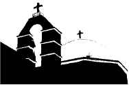
The resulting image of edge detection using Sobel operator on Figure 2 is shown in Figure 6.
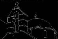
Edge detection’s result - Sobel.
In summary, this technique estimates the gradient of an image in a pixel by the vector sum of the four possible estimates of the single central gradients (each single central gradient estimated is a vector sum of vectors orthogonal pairs) in a 3×3 neighborhood. The vector sum operation provides an average over the directions of gradient measurement. The four gradients will have the same value if the density function is planar throughout the neighborhood, but any difference refers to deviations in the flatness of the function in the neighborhood 65.
4.2. Canny operator
This edge detection algorithm is very popular and attempts to find edges looking for a local maximum gradient in the gradient direction 70. The gradient is calculated by the derivative of the Gaussian filter with a specified standard deviation σ to reduce noise. At each pixel the local gradient
This method detects both strong and weak edges (very marked), and it uses two thresholds (T1 and T2 such that T1 < T2). The hard edges will be those who are superior to T2 and will be weak edges those who are between T1 and T2. Then, the algorithm links both types of edges but just considering as weak edges those connected to strong edges. This would ensure that those edges are truly weak edges 8.
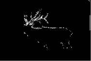
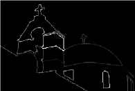
The resulting image of edge detection using Canny operator on Figure 2 is shown in Figure 7.
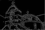
Edge detection’s result - Canny.
Summarizing, edge detection techniques use a gradient operator, and subsequently evaluate through a predetermined threshold if an edge has been found or not 71. Therefore, edge detection is a process by which the analysis of an image is simplified by reducing the amount of processed information, and in turn retaining valuable structural information on object edges 70. A more detailed analysis on edge detection techniques can be obtained in 5.
5. Fuzzy edge detection
Frequently, the edges detected through an edge detection process (as those previously presented) are false edges because these classics methods are sensitive to various issues such as noise or thick edges, among others, and require a great amount of calculation, so that discretization may present problems 64,72.
Fuzzy logic has proved to be well suited to address the uncertainty characterizing the process of extracting information from an image 73. Hence, many algorithms have included fuzzy logic in the entire process or at any particular stage of the image processing 72. An overview of models and methods based on fuzzy sets for image processing and image understanding can be found in 74.
A first idea for applying fuzzy logic in edge detection was proposed by Pal and King 75. Subsequently, Russo 76 designed fuzzy rules for edge detection. Different algorithms were created to address fuzzy edge detection since then.
Fuzzy edge detection detects classes of pixels corresponding to the variation in level of gray intensity in different directions. This is achieved by using a specified membership function for each class, in such a way that the class assigned to each pixel corresponds to the highest membership value 64. Russo 76 proposed that an efficient way to process each pixel of the image must consider the set of neighboring pixels belonging to a rectangular window, called fuzzy mask.
Let K be the number of gray levels in an image, the appropriate fuzzy set to process that image are made up of membership functions defined in the universe [0,...,K − 1] 76. Fuzzy sets are created to represent the intensities of each variable and they are associated to the linguistic variables “black” and “white”.
The resulting image of applied fuzzy edge detection on Figure 2 is shown in Figure 8.
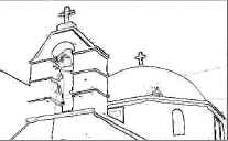
Fuzzy edge detection’s result.
The fuzzy rules used to fuzzy inference system for edge detection consist on “coloring a pixel white if it belongs to a uniform region. Otherwise, coloring the pixel black”:
- (i)
IF Ix is zero and Iy is zero THEN Iout is white
- (ii)
IF Ix is not zero or Iy is not zero THEN Iout is black.
As we mentioned previously, there are several versions of fuzzy edge detection algorithms in the literature. For instance, there is an algorithm that uses Epanechnikov function extended as a membership function for each class to be assigned to each pixel 64, or another algorithm which uses operators that detect specific patterns of neighboring pixels for fuzzy rules 77. A study about representing the dataset as a fuzzy relation, associating a membership degree with each element of the relation is presented in 78. Other issue is that fuzzy logic can be used only on a certain part of the edge detection process 72.
Fuzzy edge detection problems in which each pixel has a degree of membership to the border can be seen in some studies 79,80,81,82,83. Moreover, in these studies the concept of fuzzy boundary have been introduced.
6. Image segmentation
Around 1970, image segmentation boomed as an advanced research topic. In computer vision, image segmentation is a process that divides an image into multiple segments, in order to simplify or modify the representation of the image to be more meaningful and easy to analyze 84. Actually, there are many applications of image segmentation 85, as it is useful in a robot vision 86, detection of cancerous cells 87, identification of knee cartilage and gray matter/white matter segmentation in MR images 88, among others.
The goal of segmentation is subdividing an image into regions or non-overlapping objects with similar properties. For each pixel, it is determined whether it belongs to an object or not, producing a binary image. The subdivision level is dependent on the problem to be solved. Segmentation stops when the objects of interest have been identified and isolated. However, in most cases, processed images are not trivial and hence the segmentation process becomes more complicated.
The most basic attribute for segmentation is the intensity of a monochrome image and the color components for a color image, as well as objects boundaries and texture, which are very useful. In summary, the regions of a segmented image should be uniform and homogeneous with regard to some property such as color, texture, intensity, etc 84,89. Also, the quality of the segmentation depends largely on the output. However, although image segmentation is an essential image processing technique and has applications in many fields, there is no single method applicable to all kinds of images. Current methods have been classified according to certain characteristics of their algorithms 84,90.
Formally, image segmentation can be defined as a process of partitioning the image into a set of non-intersecting regions such that each group of connected pixels is homogeneous 85,91. It can be defined as follows:
Image segmentation partitions an image R in C subregions R1,R2,...,RC for a uniformity predicate P, such that the following items are satisfied:
- (i)
- (ii)
Ri ∩ Rj = ∅ for all i and j, i ≠ j.
- (iii)
P(Ri) = TRUE for all i = 1,2,...,C.
- (iv)
P(Ri ∪ Rj) = FALSE for any pair of adjacent regions Ri and Rj.
- (v)
Ri is connected, i = 1,2,...,C.
The first condition states that the segmentation must be complete, i.e., the union of the segmented regions Ri must contain all pixels in the image. The second condition indicates that regions have to be disjoint, that is, that there is no overlap between them. The third condition states that pixels belonging to the same region should have similar properties. The fourth condition states that pixels from adjacent regions Ri and Rj differ in some properties.Finally, the fifth condition expresses that each region must be connected 8.
Next sections describe main methods of image segmentation. They are classified into four categories: thresholding methods (6.1), watershed methods (6.2), region segmentation methods (6.3) and graph partitioning methods (6.4).
6.1. Thresholding methods
Thresholding 92 is considered one of the simplest and most common techniques that has been widely used in image segmentation. In addition, it has served in a variety of applications such as object recognition, image analysis and interpretation of scenes. Its main features are that it reduces the complexity of the data and simplifies the process of recognition and classification of objects in the image 93.
Thresholding assumes that all pixels whose value, as its gray level, is within a certain range belong to a certain class 94. In other words, thresholding methods separate objects from the background 7. So, according to a threshold, either preset by the researcher or by a technique that determines its initial value, a gray image is converted to a binary image 84. An advantage of this procedure is that it is useful to segment images with very bright objects and with dark and homogeneous backgrounds 33,100.
Let f(x, y) be a pixel of an image I with x = 1,...,n and y = 1,...,m and B = {a, b} be a pair of binary gray levels. Then, the pixel belongs to the object if and only if its intensity value is greater than or equal to a threshold value T, and otherwise it belongs to the background 8,33. The resulting binary image of thresholding an image function at gray level T is given by:
In this way, the main step of this technique is to select the threshold value T, but this may not be a trivial task at all 84. However, many approaches to obtain a threshold value have been developed, as well as a number of indicators of performance evaluation 93. For example, threshold T can remain constant for the entire image (global threshold), or this may change while it is classifying the pixels in the image (variable threshold) 33. Hence, some thresholding algorithms lie in choosing the threshold T either automatically, or through methods that vary the threshold for the process according to the properties of local residents of the image (local or regional threshold) 8,84. Some algorithms are: basic global thresholding 95, minimum error thresholding 96, iterative thresholding 97, entropy based thresholding 98 and Otsu thresholding 99.
According to Sezgin and Sankur 7, thresholding techniques can be divided into six groups based on the information the algorithm manipulates:
- (i)
Histogram shape-based techniques 100, where an analysis of the peaks, valleys and curvatures of the histogram is performed.
- (ii)
Clustering-based methods 101, where the gray levels are grouped into two classes, background and object, or alternatively they are modeled as a mixture of two Gaussians.
- (iii)
Entropy-based techniques 102, in which the algorithms use the entropy of the object and the background, the cross entropy between the original binary image, etc.
- (iv)
- (v)
Spatial techniques 105, using probability distributions and/or correlations between pixels.
- (vi)
Local techniques 106, which adapts the threshold value at each pixel according to the local characteristics of the image.
Possibly, the most known and used thresholding techniques are those that focus on the shape of the histogram. A threshold value can be selected by inspection of the histogram of the image, where if two different modes are distinguished then a value which separates them is chosen. Then, if necessary this value is adjusted by trial and error to generate better results. However, updating this value by an automatic approach can be carried out through an iterative algorithm 8:
- (i)
An initial estimate of a global threshold T is performed.
- (ii)
The image is segmented by the T value in two groups G1 and G2 of pixels, resulting from Eq. (8).
- (iii)
The average intensities t1 and t2 for the two groups of pixels are calculated.
- (iv)
A new threshold value is calculated:
- (v)
Repeat steps 2 to 4 until subsequent iterations produce a difference in thresholds lower than a given sensibility or precision (ΔT).
- (vi)
The image is segmented according to the last value of T.
Therefore, the basic idea is to analyze the histogram of the image, and ideally, if two dominant modes exist, there is a remarkable valley where threshold T will be in the middle 84. However, depending on the image, histograms can be very complex (e.g., having more than two peaks or not obvious valleys), and this could lead this method to select a wrong value. Furthermore, another disadvantage is that only two classes can be generated, therefore, the method is not able to be applied in multispectral images. It also does not take into account spatial information in the image, so it makes the method sensitive to noise 33.
The histogram of Figure 2 is shown in Figure 10. The threshold value is 170,8525.
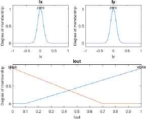
Membership functions of the inputs/outputs.
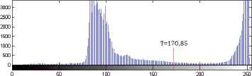
Histogram.
The outcome of thresholding to the previous image is shown on Figure 11.

Thresholding’s result.
In general, thresholding is considered to be a simple and effective tool for supervised image segmentation. It however must achieve an ideal value T in order to segment images in objects and background. More detailed studies can be found in 7,107,108,109.
6.2. Watershed methods
Watershed 110 was introduced in the field of digital topography. This method considered a grayscale picture as topographic reliefs 111,112,113,114. Later, this notion was studied in the field of image processing 115. Watershed aims to segmenting regions in catchments, i.e., in an area where a stream of conceptual water bounded by a line trickles through the top of the mountains, which decomposes the image into rivers and valleys 116. Light pixels can be considered the top of the mountain, and dark pixels to be in the valleys 117. The gradient is treated as the magnitude of an image as a topographic surface 84. Thus, it is considered that a monochrome image is a surface altitude where the pixels of greater amplitude or greater magnitude of intensity gradient correspond to the points of the river, i.e. the lines of the watershed that form the boundaries of the object. On the other hand, the pixels of lower amplitude are referred to as valley points 84,89.
By leaving a drop of conceptual water on any pixel from an altitude, this will flow to a lower elevation point until reaching a local minimum. And in turn, the pixels that drain to a common minimum, form a retention gap characterizing a region of the image. Therefore the accumulations of water in local minima neighborhood form such catchments. So, the points belonging to these basins belong to the same watershed 89. Thus, an advantage of this method is that it first detects the leading edge and then calculates the basins of the detected gradients 84.
Overall, the watershed algorithm is as follows:
- •
Calculate curvature of each pixel.
- •
Find the local minima and assign a unique label to each of them.
- •
Find each flat area and classify them as minimum or valley.
- •
Browse the valleys and allow each drop to find a marked region.
- •
Allow remaining unlabeled pixels fall similarly and attach them to the labeled regions.
- •
Join those regions having a depth of basin below a predetermined threshold.
There are different algorithms to calculate the watershed, depending on how to extract the mountain rims from the topographic landscape. Two basic approaches can be distinguished in the following subsections.
6.2.1. Rainfall approximation
The rainfall algorithm 118 is based on finding the local minima of the entire image, which are assigned a unique label. Those that are adjacent are also combined with a unique tag. Then a drop of water is placed in each pixel without label. These drops will flow through neighboring lower amplitudes to a local minimum assuming the value of the label. Then local minimum pixels are shown in black and the roads of every drop to the local minimum are indicated by white 89.
6.2.2. Flooding approximation
The flooding algorithm 110 extracts the mountain rims by gradually flooding the landscape. The flood comes from below, through a hole in each minimum of the relief and immerse the surface in a lake entering through the holes while it fill up the various catchment basins 119. In other words, the method involves placing a water fountain in local minima, then the valleys are submerged with water and each catchment filled until it reaches almost to overflow, which will create a reservoir in which neighbors are connected by the ridge 89,117. This approach comes from the bottom up to find the watershed, i.e., it starts from a local minimum, and each region is flooded incrementally until it connects with its neighbors 116.
By performing the procedure of watershed, image transform complement of Figure 1, is as shown in Figure 12.
Transform complement of binary image.
In Figure 13 is shown the outcome of watershed.

Watershed’s result.
In summary, watershed is a very simple and advantageous technique for real-life applications, mainly for segmenting grayscale images troubleshooting, and which uses image morphology 84,117. Notably, because of this method finds the basins and borders at the time of use to segment images, the key lies in changing the original image in an image where the basins correspond to objects you want to identify. Also, when it is combined with other morphological tools, watershed transformation is at the basis of extremely powerful segmentation procedures 115,120.
A critical review of several definitions of the watershed transform and their algorithms, can be found in 121,122.
6.3. Region segmentation methods
In this section, we present two region segmentation methods. These techniques try that neighboring pixels with similar properties are in the same region, i.e., they focus on groups of pixels that have similar intensity 71,94. This leads to the class of algorithms known as region growning and split and merge, where the general procedure is to compare a pixel with its neighbors, and if they are homogeneous then they are assigned to the same class 94. Region growning and split and merge are presented in section 6.3.1 and section 6.3.2 respectively.
6.3.1. Region growning
Region growning 123 is a method for grouping neighboring pixels in segmented regions according to predefined criteria of growth. Firstly, it specifies small sets of initial pixel called seed points. From them, the regions grow by adding neighboring pixels with similar predefined properties, until no more pixels that meet the criteria for inclusion in the regions are found and all pixels in the image have been scanned 8,33. Similarly, if two or more regions are homogeneous, they are grouped into one. Also, once a region has no more similar pixels, then we proceed to establish a new region from another seed 124.
In summary, the basic procedure is presented bellow 33:
- •
Select a seed group of pixels in the original image.
- •
Define true value criterion for the stopping rule.
- •
Combine all pairs of spatially adjacent regions fulfilling the criterion value.
- •
Stop the growth of the regions when it is not possible to combine more adjacent pixels.
However, a disadvantage of this method is the fact that getting a good result depends on the selection of the initial seed points and the order in which they are scanned for grouping each pixel. This dependence makes the segmented result to be sensitive to the location and ordering of seeds 71,89.
The resulting image of region growing on Figure 2 by applying a seed in the pixel x = 148 y = 359, is shown in Figure 14.
Region growing’s result.
Consequently, region growing is a procedure which iteratively groups pixels of an image into sub-regions according to a predefined criterion of homogeneity from a seed 33,124. Similarly, region growning has a good performance because it considers the spatial distribution of the pixels 124.
6.3.2. Split and merge
Split and merge 71 is based on a representation of data in a quadtree where if a region of the original image is non-uniform in attribute then a square image segment is divided into four quadrants. Hence, if four neighbors are uniform, they are united in a square formed by these adjacent squares 89.
Definition 1.
Let I be an image and P be a predicate, the image is subdivided into small quadrants, such that for any region Ri it is P(Ri) = TRUE. If P(R) = FALSE, the image is divided into quadrants. If P is FALSE for any quadrant, the quadrant is subdivided into sub-quadrants, and so on.
This process is represented by a tree with four leaves descendants called quadtree, where the root refers to the initial image and each of its nodes represent its four subdivisions 8.
The procedure is as follow 8,33:
- (i)
Start with the complete image, where R represent the entire image region, if P(R) = FALSE.
- (ii)
The entire image R is divided into four disjoint quadrants, and if P is false for any quadrant (P(Ri) = FALSE), then the quadrants are subdivided into sub-quadrants until no more splits are possible.
- (iii)
Once no more splits can be done, any adjacent regions Ri and Rj for which P(Ri ∪ Rj) = TRUE are joined together.
- (iv)
The process ends once further connections are not possible.
Thus, split and merge arbitrarily subdivides an image into disjoint regions, and then these regions are joined or divided according to the conditions of image segmentation in Section 6. This method performs well when the colors of objects in the image are not very opposite.
The resulting image of split and merge on Figure 15 is shown in Figure 16.
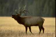
RGB image 9.
Split and merge’s result.
Generally speaking, split and merge begins with nodes (squares) at some level of the quadtree, so if a quadrant is not uniform a split is done, being subdivided into four sub-quadrants. However, if four adjacent quadrants are uniform, a merge between them is performed 71.
Besides, it is important to mention that the main advantage of region segmentation based techniques is that they attempt to segment an image into regions quickly, because the image is analyzed by regions and no by pixels.
6.4. Graph partitioning methods
A digital image I is modeled as a valued graph or network composed by a set of nodes (υ ∈ V) and a set of arcs E (e ∈ E ⊆ V ×V) that link such nodes 125,126,127. Graphs have been used in many segmentation and classification techniques in order to represent complex visual structures of computer vision and machine learning. In this section algorithms which use graph are presented, but first a formal proposition is shown.
Proposition 1.
If A digital image I is viewed as a graph where the nodes are the pixels, let V = {P1, P2,...,Pn} be a finite set of pixels in the image and let E{{Pa, Pb}|Pa, Pb ∈ V} be unordered pairs of neighboring pixels. Two pixels are neighbors if there is an arc eab = {Pa, Pb} ∈ E. Let G = (V, E) be the representation of neighboring relations between the pixels in an image. Let also dab ⩾ 0 be the degree of dissimilarity between pixels Pa y Pb. Let D = {dab|eab ∈ E} be the set of all the dissimilarities. Let N(I) = {G = (V, E);D} be the network which summarizes all the previous information about an image I.
With the above proposition, it is possible to extract meaningful information about the processed image, checking the various properties of the graphs. As we shall see throughout this section, the graphs turn out to be extremely important and useful tools for image segmentation. Some of the most popular graph algorithms for image processing are presented next.
6.4.1. Random walker
A random walker 128 approach can be used for the task of image segmentation through graphs: a user interactively label a small number of pixels called seeds, and each of the not labeled pixels releases a random walker, so the probability is calculated when the random walker reaches a labeled seed 129. This algorithm may be useful for segmenting an image in, for example, object and background, from predefined seeds indicating image regions belonging to the objects. These seeds are labeled, and unlabeled pixels will be marked by the algorithm using the following approach: let a random walker start on an untagged pixel, what is the probability that arrives first at each seed pixel?. A K − tuple vector is assigned to each pixel, which specify the probability that a walker beginnings in an unlabeled pixel, first reaches each seed point K. Then, from those of K −tuples it is selected the more likely seed for the random walker 127.
The random walker algorithm consist of four steps 127:
- •
Represent the image structure in a network, defining a function that assigns a change in image intensities, so assign the weights of the edges in the graph.
- •
Define the set of K labeled pixels to act as seed points.
- •
Solve the Dirichlet problem for each label except the last, which is equivalent to calculate the probability that a random walker beginning from each unlabeled pixel reaches first each of the K seed pixels.
- •
Select from these K −tuples the more likely seed for the random walker, that is, assign each node υi to the maximum probability label.
The algorithm above consists in generating the graph weights, establishing the system of equations to solve the problem and implement the practical details. Several properties of this algorithm are quick calculation, rapid editing, inability to produce arbitrary segmentation with sufficient interaction and intuitive segmentation 127. Moreover, an advantage is that the edges of faint objects are found when they are part of a consistent edge 130.
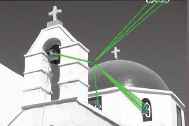
The resulting image of random walker on Figure 3 is shown in Figure 17. Notice that this figure shows the two selected seeds (K = 2), green and blue, as well as the probability that a random walker released at each pixel reaches the foreground seeds. That is, the near the green seed are the nearest objects so their color is similar to the pixel where seed is. Similarly, blue seed is surrounded of other color and its color is more similar. The intensity of the color represents the probability that a random walker leaving the first pixel reaches each seed.

Random walker’s result.
Random walker contributes as a neutral technique for image segmentation because it does not consider any information of the image. Instead, the segmentation is derived from the K −tuples of each pixel, selecting the most probable seed for each pixel or random walker 130.
6.4.2. Graph cuts
Graph cuts 131 is a multidimensional optimization tool that is capable of applying smoothing in pieces, while maintaining marked discontinuities 132. It is supported in both graph theory and the problem of minimizing the energy function, uses the maximum flow problem within graph. Thus, through the max-flow min-cut theorem, it is defined the minimum cut of the graph, such that the cut size is not larger in any other cut 133.
A s-t cut is a subset of arcs C ∈ E such that the S and T terminals are completely separated in the induced graph G(C) = (V, E\C) 134.
Definition 2.
A s-t cut or simple cut of a graph G = (V, E) is a binary partition of nodes V into two subsets with a primary vertex in each: source S and sink T = V − S such that s ∈ S and t ∈ T 132,135.
Thus, each graph has a set of edges E with two types of terminal nodes P: n − links, referring to non-terminal neighboring arcs; and t − links, that are used to connect terminal pixels to non-terminal pixels. Each graph edge is assigned some nonnegative weight or cost w(p, q), so a cost of a directed edge (p, q) may differ from the cost of the reverse edge (q, p). The set of all graph edges consist of n − links in N and t − links {(s, p), (p, t)} for non-terminal nodes p ∈ P 132,134.
The minimum cut problem is based on finding the cut with the minimum cost among all cuts. The cost of a cut C = (S,T) is the sum of the costs/weights of the arcs borders (p, q) such that p ∈ S and q ∈ T. Thus, the min-cut and max-flow problems are equivalent, because the maximum flow value is equal to the cost of the minimum cut 132,136,137.
If f is a flow in a graph G with two terminal nodes called source s and sink t, respectively representing “object” and “background” labels, and a set of non-terminals P nodes, then the value of the maximum flow is equal to the capacity of a minimum cut C 132,134,135.
The basic algorithm for this procedure developed by Boykov and Kolmogorov 133 based on increasing paths through two search trees for the terminal nodes, consists of three steps that are iteratively repeated:
- •
Growth phase: search trees S and T grow until they touch giving an s → t path.
- •
Augmentation phase: the found path is augmented, search tree(s) break into forest(s).
- •
Adoption phase: trees S and T are restored.
Other max-flow min-cut algorithms are based on the push-relabel methods, which are based on two basic operations: push flow and relabel from an overflowing node 135.
In general, the cut may generate a binary segmentation with arbitrary topological properties 134. For example, if you work with the observed intensity I(p) of a pixel p, a cut would symbolize a binary labeling process f, which assigns labels fp ∈ {0,1} to the pixels in such a way that if p ∈ S then fp = 0 and if p ∈ T then fp = 1 132.
One advantage of this method is that it allows a geometric interpretation, and also works with a powerful tool for the energy minimization (a binary optimization method). There are a lot of techniques based on graph cuts that produce good approximations. This technique is used in many applications as an optimization method for low vision problems, based on global energy formulations. In addition, graph cuts can be very efficient computationally, and this is why they provide a clean, flexible formulation of image segmentation 132.
Frequently, this method is combined with others, however, an improved graph cut method named normalized cuts 138 is based on modifying the cost function to eliminate outliers. The usage of this technique within image processing context is presented in the following section.
6.4.3. Normalized cuts
This procedure works with weighted graphs G = (V, E) where the weight w(i, j) of each arc is a function of the similarity between nodes i and j 139.
A graph G = (V, E) is optimally divided into two disjoint subsets A and B with A ∪ B = V and A ∩ B = ∅ when Ncut value is minimized. The degree of dissimilarity of A and B is measured as a fraction of the total weight of the connections arcs on all nodes in the network. This is called normalized cut (Ncut) 139:
The total normalized association measure within a group for a given partition is expressed as 139:
Given a partition of nodes of graph V into two disjoint complementary sets A and B, let x be an N = |V| dimensional indication vector, xi = 1 if node i is in A and xi = −1 otherwise. Also, let
The algorithm can be summarized in the following steps 138,139:
- •
Given an image, represent it in a weighted graph G = (V, E), and summarize the information into W and D (let D = diag(d1, d2,...,dN be an N ×N diagonal matrix and W be an N × N symmetric matrix with W(i, j) = wij).
- •
Solve (D −W)x = λDx for the eigenvectors with the smallest eigenvalues.
- •
Use the eigenvector with the second smallest eigenvalue to subdivide the graph by finding the splitting points to minimize Ncut.
- •
Check whether it is necessary to split the current partition recursively by checking the stability of the cut.
- •
Stop if for any segment Ncut exceeds a specified value.
The resulting image of gray-scale image segmentation using normalized graph cuts on Figure 2 is shown in Figure 18.
Normalized cuts’s result.
Thus, the normalized cuts method originated because if we only consider to minimizing the cut value
6.4.4. Region adjacency graphs
Region adjacency graphs (RGA) 71 provides a spatial view of the image, in order to efficiently manipulate the information contained in it, through a graph which associates a region and the arcs linking each pair of adjacent regions with each vertex 124.
A region Ri defined by a quadruple Ri = (k, xk, yk, Ak)|k ∈ (1,...,n), where k refers to the index number of the region, (xk, yk) represents the center of gravity and Ak represents the area.
A RAG is defined by a set of regions and a set of pairs of regions: ({Ri},{(Rj, Rk)} | i, j, k ∈ (1,...,n)). Thus, the set of parts described all regions involved. And the set of pairs of regions indicate regions which are adjacent 140.
As we mentioned above, nodes represent the regions and are compared in terms of a formulation based on chains. Thus, a region can be perceived as a shape whose boundary is represented by a cyclic chain (boundary string), which consists of a sequence of simple graph arcs. According to a given algorithm, the similarities between two border chains are calculated 126.
Two important characteristics of the RAG raised by Pavlidis 71 are:
- (i)
The degree of a node is the number of adjacent regions to a given region, which usually is proportional to the size of the region.
- (ii)
If a region completely surrounds other regions, that node is a cutnode in RAG, as shown in the following figure.
Despite being a very useful and robust tool, this method has the disadvantage that it does not produce good results when the processed image has not perfectly defined regions or discontinuities 141.
The resulting image of RAG on Figure 2 is shown in Figure 20. The algorithm uses watershed algorithm to find structure of the regions in the image. Then, two regions are considered as neighbors if they are separated by a small number of pixels in horizontal or vertical direction.
Example of region adjacency graph 71.
Region adjacency graph’s result.
Accordingly, this technique is used to provide an efficient system for manipulating implicit information in an image through a spatial view. So each node in the RAG represents a region, and two nodes (regions) are linked if they are neighbors 142.
Summarizing, graph theory has the advantage of organizing the image elements into mathematically sound structures making the formulation of the problem more understandably and enabling less complex computation 143.
The image segmentation techniques presented in this section have been categorized into four classes: thresholding methods, watershed methods, region segmentation methods and graph partitioning methods. In addition, some evaluation methods are created to evaluate quality of an image segmented. A review of these evaluation methods for image segmentation is presented in 144,145.
7. Hierarchical image segmentation
Hierarchy theory 146 has been frequently used in sociology and anthropology. These sciences study a hierarchical set of social classes or strata 147. In this section, we present the definition of hierarchical segmentation methods, which try to group individuals according to criteria starting from one group including all individuals until creating n groups each containing a unique individual. This can be done in two ways, by agglomerative methods 148 or by divisive methods 149, where the groups are represented by a dendrogram based on a two-dimensional diagram as a hierarchical clustering 4.
The agglomerative methods are responsible for successively merge the n individuals in groups. On the other hand, the divisive methods choose to separate the n individuals into progressively smaller groupings.
First, we begin by presenting the elements needed to obtain a hierarchical image segmentation using graphs.
According to Gómez et al. 150,151 given an image I and its network N(I), a family S = (S0, S1,...,SK) of segmentations of N(I) constitute a hierarchical image segmentation of N(I) when the following properties are verified:
- •
St ∈ Sn(N(I)) for all t ∈ {0,1,...,K}, (i.e., each St is an image segmentation of N(I)).
- •
There are two trivial partitions, the first S0 = {{v}, v ∈ V} containing groups with one node (singleton), and another partition SK = {V} containing all pixels in the same cluster.
- •
|St| > |St+1| for all t = 0,1,...,K − 1, indicating that in each iteration the number of groups or communities increases.
- •
One advantage of hierarchical segmentation is that it can produce an ordering of the segmentations, which may be informative for picture display. So in any hierarchical image segmentation proceedings, no apriori information about the number of clusters is required. A dendrogram helps in making the selection of the number of groups on the same levels. The partitions are achieved through the selection of one of the solutions in the nested sequence of clusters making up the hierarchy. The best partition is at a certain level, where the groupings below this height are far apart.
Another advantage of hierarchical segmentation is that it can be used to build fuzzy boundaries by a hierarchical segmentation algorithm designed by the authors 150,152,153,154,155,156.
There are some algorithms of hierarchical image segmentation, as 158,159,160,161,162 among others. In the next subsection, we present an algorithm of hierarchical image segmentation based on graphs.
7.1. Divide & link algorithm
The divide-and-link (D&L) algorithm proposed by Gómez et al. 155 and extended in 156 is a binary iterative unsupervised method that obtains a hierarchical partition of a network, to be shown in a dendrogram, and it is framed as a process to partition networks through graphs.
Generally speaking, D&L tries to group a set of pixels V of a graph G = (V, E) through an iterative procedure that classifies nodes in V in two classes V0 and V1. However, the rating depends on the type of edge. There are endpoints of division edges that are assigned in different classes (split nodes) and there are endpoints of link edges that are assigned in the same class (link nodes).
The D&L algorithm consists on the following main steps 150:
- (i)
Calculate the division and link weights for each edge.
- (ii)
Organize subgraph edges Gt sequentially according to the weights of the previous step.
- (iii)
Build a spanning forest Ft ⊂ Gt (through, for instance, a Kruskal-like algorithm 163) based on the arrangement found in the previous step.
- (iv)
Build a partition Pt following the binary procedure applied to Ft.
- (v)
Define a new set of edges Et+1 from Et by removing those edges that connect different groups of Pt.
- (vi)
Repeat steps i–v while Et+1 = ∅.
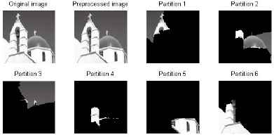
The output of the D&L algorithm (with six partitions) applied to Figure 3 is shown in Figure 21.

D&L’s result.
In summary, any hierarchical image segmentation algorithm is a divisive process because it starts with a trivial partition, formed by a single group containing all nodes, and ends with another trivial partition formed by as many groups as nodes possesses the finite set of elements you wish to group. It also has a polynomial time complexity and a low computational cost. One advantage is that it can be used in a variety of applications.
8. Fuzzy image segmentation
Fuzzy image segmentation concept was introduced in 151,156 and extended in 150,157, where they established that a fuzzy image segmentation should be a set of fuzzy regions R1,...,Rk of the image. They presented a way to define this concept based on the fact that crisp image segmentation can be characterized in terms of the set of edges that separates the adjacent regions of the segmentation.
Definition 3.
Given an image modeled as a network image N(I) = {G = (V, E); D}, a subset B ⊂ E characterizes an image segmentation if and only if the number of connected components of the partial graph generated by the edges E − B, denoted as G(E − B) = (V, E − B), decreases when any edge of B is deleted.
In this sense, a formal definition of fuzzy image segmentation is through the fuzzyfication of the edge-based segmentation concept introduced in Definition 3 of this section (see 150 for more details).
Definition 4.
Given a network image N(I) = {G = (V, E); D}, we will say that the fuzzy set
In the previous definition, the membership function of the fuzzy set
In 157, it has proven that there exist a relation between fuzzy image segmentation concept and the concept of hierarchical image segmentation. In that paper, it is showed that it is possible to build a fuzzy image segmentation from a hierarchical image segmentation in the following way.
Given a network image N(I) = {G = (V, E);D}, let ℬ = {B 0 = E, B 1,...,BK = ∅} be a hierarchical image segmentation, and for all t ∈ {0, 1,...,K} let μt : E → {0,1} be the membership function associated to the boundary set Bt ⊂ E. Then, the fuzzy set
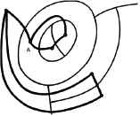
The output of fuzzy image segmentation applied to Figure 3 is shown in Figure 22. In this picture has been aggregated the output of hierarchical image segmentation of Section 7.1, in order to build a fuzzy image segmentation 157.
Fuzzy image segmentation’s result.
9. Final remarks
The main characteristics and relationships between some of the best known techniques of digital image processing have been analyzed in this paper. These techniques have been classified according to the output which they generate, and attending to the problems they face. Also, this classification depends on whether they are supervised or unsupervised methods, and whether they are crisp or fuzzy techniques. In this way we can notice that different problems should be formally distinguished when trying to recognize an object in a digital image (such as classification, edge detection, segmentation and hierarchical segmentation). For example, it has been pointed out that the output of an edge detection problem does not necessarily produce a suitable image segmentation. Edge detection only detects the border of the objects and does not necessarily separate objects in the image.
Furthermore, some of the techniques reviewed in this paper can be used as a previous step for another technique. For example, an edge detection output could be the input for an image segmentation if we find a partition of the set of pixels into connected regions. The opposite is also true, and it is possible to find the boundary of a set of objects through the set of pixels that connect pixels of different regions. Also, in an output of image segmentation, if two different and not adjacent subsets of pixel can share the same characteristics, we can apply an image classification technique and then these regions will belong to the same class. Moreover, a solution of clustering can be a previous step to reach an image segmentation. Thus, although different, these techniques can be related to each other.
Computational intelligence is a must in a wide range of challenging real-world image processing problems. More sophisticated original approaches, variations and combinations should be expected depending on the specific characteristics of each image and the decision-maker objectives (see, for example 164). In particular, one of the most important applications of computational intelligent techniques is the imaging process which is used in many fields as for example, digital imaging 165, medical imaging 166, industrial tomography 167, chemical imaging 168 and thermography 169.
We would like to remark that there were found no significative differences in computational time when processing all the images considered in this paper with different algorithms, being in general quite short.
Finally, it is important to point out that in the background of an edge detection process, there is a classification problem, because a pixel is classified as either edge or not edge. Similarly, a thresholding method can be a classification problem because a pixel is classified as either object or background. In this manner, the classification of the methods shown in this paper can be extended even more generally, a problem to be considered in a future research.
Acknowledgments
This research has been partially supported by the Government of Spain, grant TIN2015-66471-P, and by the Government of the Community of Madrid, grant S2013/ICE-2845 (CASI-CAM-CM).
References
Cite this article
TY  - JOUR
AU  - C Guada
AU  - D Gómez
AU  - JT. Rodríguez
AU  - J Yáñez
AU  - J Montero
PY  - 2016
DA  - 2016/04/01
TI  - Classifying image analysis techniques from their output
JO  - International Journal of Computational Intelligence Systems
SP  - 43
EP  - 68
VL  - 9
IS  - Supplement 1
SN  - 1875-6883
UR  - https://doi.org/10.1080/18756891.2016.1180819
DO  - 10.1080/18756891.2016.1180819
ID  - Guada2016
ER  -