
Numeric Character Recognition System for Chilean License Plates in semicontrolled scenarios
- DOI
- 10.2991/ijcis.2017.10.1.28How to use a DOI?
- Keywords
- Artificial Vision; Pattern Recognition; Optical Character Recognition; Fine Character Segmentation
- Abstract
The development of a computational tool for the recognition of numerical characters already segmented from Chilean license plates, located in semi-controlled scenarios, is presented. Two algorithms are highlighted: one for the Fine Segmentation of the Characters through the K-Means algorithm and a system of fuzzy logic; and a second one for the recognition through learning of the pseudo-real outline of the characters’ skeletona. The tool has an efficacy of 95 % and a processing time of 0.4 s.
- Copyright
- © 2017, the Authors. Published by Atlantis Press.
- Open Access
- This is an open access article under the CC BY-NC license (http://creativecommons.org/licences/by-nc/4.0/).
1. Introduction
License Plate Recognition (LPR) by Optical Character Recognition (OCR) is an issue that is studied in Intelligent Transport Systems (ITS) and is important in intelligent infrastructure systems applications [1–8].
Although several OCR methods are mentioned in the specialized literature, these are generally developed for classic scenarios with plain texts (i.e. text images without perspective). Therefore, they are not applicable to real scenarios such as LPR [9].
OCR by LPR presents intrinsic difficulties that are reflected in restrictions in existing LPR systems, such as the use of relatively static scenarios, stable lighting, known distance between the plate and the camera, lens or sensor with practically invariable parameters over time, among others. This, together with current efficacy rates, shows that OCR in LPR is an issue that has not been solved completely [5, 6]. OCR methodologies in LPR vary in their complexity as a function of the restrictions mentioned above. In this context reference can be made to image comparison with templates, the use of projections [10], the use of multiple cameras [11], character outline sampling, Hotelling transform, topological characteristics of the character, among others [5, 6]. It should be pointed out that there is no consensus on the methodology used to define the efficacy of LPR, and there are various publications that do not detail the type of scenario used for image acquisition [5]. The use of comparison characteristics based on the morphology of the pseudo-real outline of the characters’ skeletona allows reducing the restrictions, because the shape of a character does not very much in spite of visual alterations. However, this solution implies a high computational cost that has led to the preferential use of other selection characteristics which, in spite of allowing an acceptable LPR, deliver little information on the real morphology of the character, giving rise to the mentioned restrictions.
The need for the recognition of numeric characters present in Chilean license plates, which is also a not properly solved matter, stems from ITS requirements for recognizing vehicles that possess license plates ending in some specific numeric character. This information is mainly used to regulate vehicles in transit during driving bans frequently related to critical environmental situations.
Ultimately, in the present work a computational tool is designed and developed for the recognition of already segmented numerical characters from Chilean or similar license plates located in semi-controlled scenarios that reduces or attenuates the restrictions by means of a classification based on learning the morphological characteristics of the outline of the characters’ skeleton.
2. Description of the System
The numerical character recognition tool was developed using MATLAB® and it allows, through computer vision, the recognition of already segmented numerical characters of license plates from digital images acquired in semi-controlled scenarios.
The method developed for the OCR, called Robust Recognition of Licence Plate Numerical Characters (RRLPNC), is based on the use of the pseudo-real outline morphology of the skeleton of the characters as classification variables.
To that end, the morphological characteristics of the skeleton are extracted first, generating a 45-element characteristics vector, and then a classification system based on learning determines whether each extracted characteristics vector (X ∈ ℝ45) belongs to one of the ten classes that define each numerical character. The stages of the developed methodology are shown in Fig. 1.
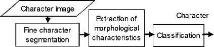
Stages of RRLPNC.
The semi-controlled scenario considered for this work makes use of digital images where there is no full control of the following characteristics: kind of lighting, type of lens, background image, distance, and plate rotation.
The images are obtained from in-situ photographs made with a photographic camera with a digital CCD sensor (5 megapixel resolution) in open spaces and from websites meant for the sale of used cars where the sellers provide their own photographs, with no control over the characteristics.
In this context, due to the impossibility of publicly accessing to a set of images containing Chilean license plates, which would allow the comparison of the developed tool, this work employs images retrieved from the aforementioned websites. Thereby, a non-arbitrary and effective dataset was obtained for the validation process of the numeric character recognition results.
It should be noted that the semi-controlled scenario considers rotation values of license plates belonging to a Δθ = 10° interval where the OCR is performed without modifying the image due to rotation.
2.1 Effective Visualization Zone and Digital Image Processing
The spatial bounding of the tool is given by the positions and orientations of the plate in relation to the capture device. For this, the Effective Visualization Zone is defined as the portion of the scenario from which the images for the OCR can be acquired. Fig. 2 shows that zone, represented as the shaded fragment of the visual field of the capture device.
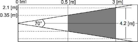
Effective Visualization Zone.
The depth of field values from 0.5 m to 3 m are determined as a function of intrinsic characteristics of the studied system, such as the actual size of the characters, the camera’s resolution and aperture angle, and operating limits generated in the design of the developed methodologies, e.g., the minimum image size of an 8x8 pixels character required by the stage meant for the extraction of morphological characteristics.
For the treatment of the digital image, it is defined that it comes from a real image modeled by IR(x, y, t, λ), where: x and y are the position components, t is the time, and λ is the wavelength of the electromagnetic signal. IR is digitized by a capture device based on electronic photocells, where the acquisition of visible electromagnetic energy is quantified as a function of the degree of capture for the wavelength of the light-capturing implement, that is:
where Si(λ) corresponds to the efficiency to the stimulus for a wavelength of the ith light capturer.
The processed digital image is represented by means of the vector function
with (i, j) ∈ ℕ /i ≤ M, j ≤ N. (ri,j, gi,j, gi,j) ∈ ℕ0/r ≤ 255, g ≤ 255 and b ≤ 255, where r, g, b are the color components in RGB, and i and j define the image’s row and column, respectively.
3. Fine Character Segmentation
The Fine Segmentation isolates the characters from elements foreign to them, such as spots. For that purpose a partition grouping algorithm is developed by means of K-Means, with K=3, and a fuzzy logic system for selecting the K-group that represents the character.
The nearness criterion that quantifies the distance between each sample represented by vector X and the centroids (vector
where (i and j) and (r, g and b) are the position and RGB color components of each sample, respectively, while the variables of the centroids are represented with an upper bar; and pi and pj are weighting values.
Fig. 3 shows the results of the grouping, where white pixels represent the data belonging to each group. Note how, in spite of the low resolution of some images or the appearance of foreign objects, the algorithm is able to classify the character’s pixels in some of the three groups.
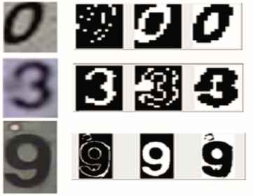
Groups obtained through K-Means.
Then the group that best represents the character is determined by analyzing four normalized selection characteristics:
- •
“Density:” ratio of the number of data contained in the group and in the original image.
- •
“Height:” ratio of the number of not null rows that the group and the original image contain.
- •
“Width:” ratio of the number of not null columns that the group and the original image contain.
- •
“Perimeter:” ratio of the number of pixels of the group that coincide in position with the perimeter of the original image and the number of pixels that constitute the image’s total perimeter.
In view of the deterministic uncertainty, when quantifying the perceptions of height, width and density, the processing of the characteristics is developed by means of a fuzzy system in which the defined fuzzy sets are represented in Table 1.
| Fuzzy variable | (Low) | Fuzzy sets (Ok) | (Height) |
|---|---|---|---|
| x1= Xheight | Bht | Oht | Aht |
| x2= Xwidth | Bwd | Owd | Awd |
| x3= Xdensity | Bden | Oden | Aden |
| x4= Xperimeter | --- | Oper | Aper |
Defined fuzzy sets.
The membership functions that quantify the fuzzy belonging of each variable to the fuzzy sets are represented in Fig. 4. Equation (4) is an illustration of the membership function that determines the belonging of the fuzzy variable Xheight to the fuzzy set Bheight.
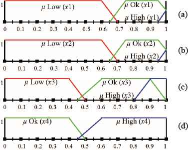
Membership functions: (a) Height, (b) Width, (c) Density, (d) Perimeter.
Then the fuzzy inference is made based on rules modeled by the following equations:
Finally, the selection of the group that belongs to the character is the one that maximizes equation (9), which defuzzifies the selected variables.
With respect to the results, the Fine Segmentation process presents an average efficacy of 99.2 % for 500 samples, achieving its objective in spite of the low resolution or quality of some of the images.
4. Extraction of Morphological Characteristics
The Extraction of Morphological Characteristics (EMC) consists of four sequential subprocesses shown in Fig. 5.
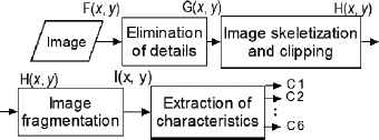
EMC process carried out.
The first two subprocesses simplify and make the image adequate to facilitate the later EMC. The elimination of details removes pixels that do not provide information for the OCR, keeping only zones that present densities higher than a threshold, in this way reducing the size of the image as shown in Fig. 6.
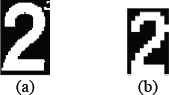
Elimination of details: (a) Original image, (b) Simplified and reduced image.
Thanks to the skeletization a continuous pattern is obtained that contains the smallest possible number of data, but retains the morphology of the original object. Fig. 7b shows the skeletization of the characters of Fig.7a made by means of the “voronoiSkel” function (supplied by MATLAB® and owned by Yohai Copyright). Finally, the image is trimmed, removing the ends that do not present skeleton pixels (see Fig. 7c).
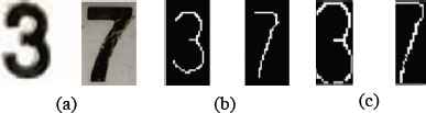
Pre-processing: (a) Original image, (b) Skeletization, (c) Trimming.
The fragmentation module divides the image into six zones of equal size (see Fig. 8).
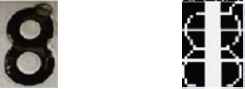
Image fragmentation.
4.1. Extraction module of morphological characteristics
The EMC module looks for and quantifies the existence and apparent shape of six predefined geometric figures in each of the zones that constitute the fragmented character, so the total morphological characteristics of the character are represented by six characteristics vectors. The morphological characteristics found in each zone are unique, i.e., no more than one figure is recognized per zone.
The type of figures to be looked for are:
- •
Vertical straight line
- •
Horizontal straight line
- •
Type c(x) = Ax3 + Bx2 + Cx + D curve
- •
Two perpendicular straight lines consisting of only vertical and horizontal segments
- •
Two non-perpendicular intersecting straight lines
- •
Empty image
To improve the efficacy of the OCR in images with perturbations that “distort” the morphology of the character, generated among others by rotation of the image, spots, etc., the figure searching methodology has a geometric tolerance that allows it to recognize the figures that have been mentioned even if they have imperfections.
The search for the six figures is made by means of sequential modules devoted to the exclusive extraction of a figure in particular, with the information obtained in each module being used for the remaining modules. Fig. 9 presents the developed modules, where CS are Corner Segments; TS are perpendicular segments whose ends do not match; and NPS are non-perpendicular Segments.

EMC.
1) Global Image Scanning: By Global Scanning characteristics that constitute configuration parameters for the following subprocesses are obtained. It is performed by two pixel reading scans, one vertical and one horizontal, calculating the normalized average distance presented by each row or column with respect to its origin given by some of the image’s vertices.
To get the normalized average distance, let us consider row vector
So the normalized average distance of
The vector function that establishes the normalized average distance for the total of m-rows that constitute the image is given by:
Fig. 10b shows
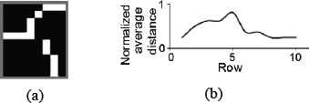
Normalized average distance: (a) Original image, (b)
2) Search Empty Image: Each zone is considered empty if its density is lower than 3 %.
3) Search Vertical Straight Line: Initially, it is confirmed whether the zone corresponds to a vertical straight line, verifying that the number of not null columns is less than 30 % of the total columns that constitute the zone. Once the existence of the vertical straight line is confirmed, a single not null column is generated in the analyzed zone that corresponds to the vertical straight line found. This is done by processing the existing not null columns, incorporating a geometric tolerance to define the morphology of the straight line using a previous knowledge base founded on the greater visual importance presented by larger objects.
With the purpose of forming a single segment for each not null column, initially the algorithm processes each not null column by eliminating or joining possible existing segments based on the quantification of its discontinuities and spatial locations. Fig. 11 shows, as an example, the results of processing columns 3, 4, and 6.
Column modification: (a) Original image, (b) Modified image.
To generate a single segment, the algorithm makes an exploratory scan in each not null column looking for and saving size and position values (upper and lower limits) of the possible existing segments.
As an example, for column four of Fig. 11a the algorithm recognizes two segments, S1 with a limup1 = 1 upper limit and a limlow1 = 1 lower limit, while segment S2 presents a limup2 = 5 and limlow2 = 7. That is, each n-possible segment found is represented by row vector
If there is more than one segment, the algorithm generates a single segment that is defined as SC, eliminating or joining the segments found according to their sizes. Considering the only exploratory scanning direction, it is concluded that limup2 > limup1 and limlow2 > limlow1. Therefore, the size of a segment in pixels is
So finally, as an example, SC for each column that has two segments will be given by
Then, by grouping the SC segments found per column, a single vertical straight line is determined for the whole zone, where the position and size of this straight line is given by:
- •
Column: the one that presents the largest SC, provided that this is not the only one that is disconnected from its SC neighbors.
- •
Upper row: equal to the upper vertical limit of the highest SC.
- •
Bottom row: equal the lower vertical limit of the SC that has the largest lower limit.
Fig. 12 shows the results when a single straight line is defined with two identified segments (SC).
Generation of vertical straight line: (a) Original image, (b) Vertical straight line.
4) Search Horizontal Straight Line: The developed methodology is similar to that used in vertical straight lines. Basically, the scanning direction and the spatial reference frame used are changed.
5) Search Curve: It is considered that the zone corresponds to a curve if there is some third degree polynomial that can model the real values of
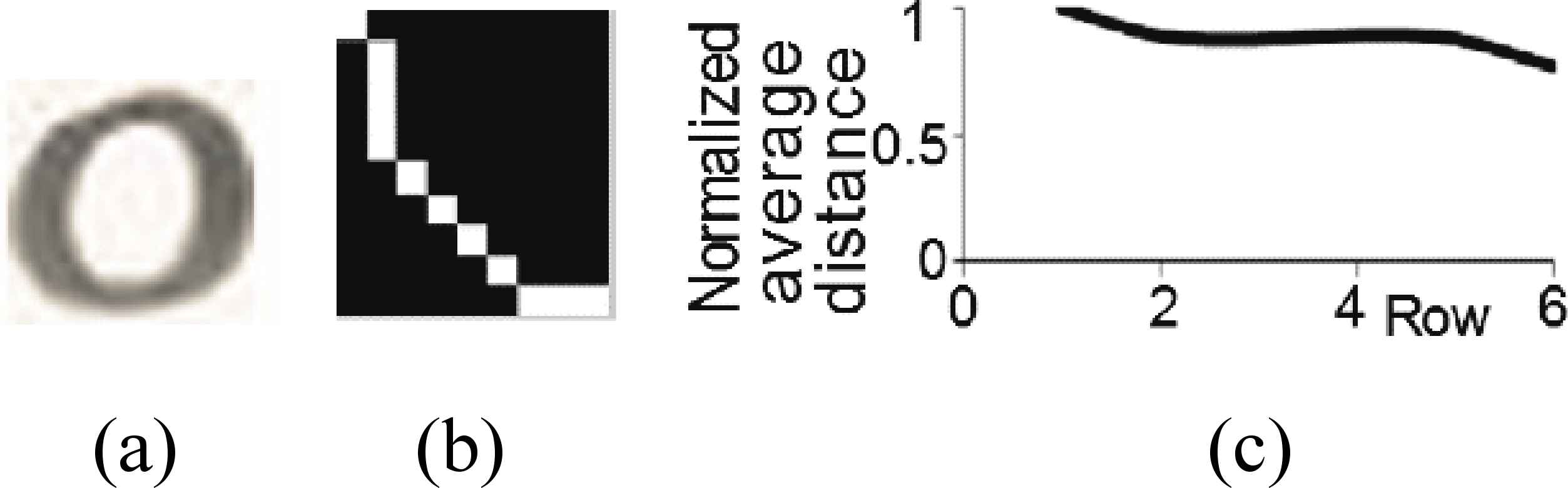
Search curve: (a) Original image, (b) Skeleton of character’s bottom left zone, (c) Found curve.
Finally, the model’s domain is identified (rows of the zone where the curve actually exists), and it is used as information for the classification.
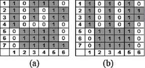
6) Search for Two Intersecting Segments: The type of intersecting segments sought correspond to those where the intersection point coincides with one of the ends of at least one of the segments (see Fig. 14). The three types of intersections sought are:
- •
“Corner Segments” (CS): formed by perpendicular segments which coincide in position at some of their ends
- •
“T Segments” (TS): Perpendicular segments none of whose ends coincide.
- •
“Nonperpendicular Segments” (NPS)
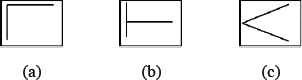
Intersections: (a) CS, (b) TS, (c) NPS.
The search is based on the fact that the existence of one of the intersections generates a maximum and/or minimum (of considerable magnitude) in
Fig. 15 presents two explicative cases of the search for CS and TS segments, showing how intersection CS of the top left zone of the character “5” (Fig. 15: a, b and c), presents a single maximum at
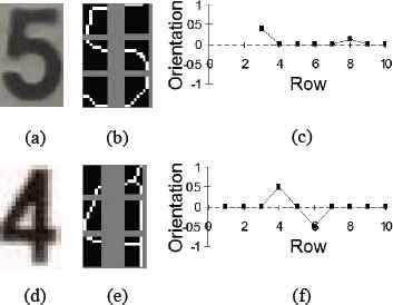
Orientation: (a and d) Original images, (b and e) Skeletons, (c and f)
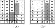
To determine the existence of CS the algorithm verifies the existence of a single maximum or minimum in
∀ i ∈ ℕ/ i = 1, 2, … , m.
After defining the existence of an CS intersection, its morphology is determined. The location of the intersection of the segments is given by points (i′, j′), where i′ is the row in which the maximum or minimum were found, and j′ is the statistical mode of
The direction of the intersection defined by the location of the ends of the segments that do not coincide with point (i′, j′) depends on whether what was found at
For the three left zones of the fragmented character, the coordinates at the ends of the vertical, Sv, and horizontal, Sh, segments that form an CS with intersection point P (i′, j′) are given by
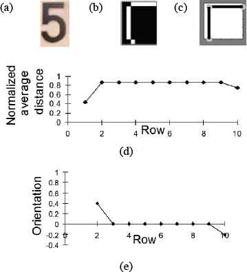
CS: (a) Character, (b) Skeleton of top left zone, (c) EMC, (d)
To determine the existence of a TS, three requirements are verified by the algorithm:
- •
- •
The original image must have a horizontal segment in the row in which the maximum or minimum was found, with a minimum length equal to one fourth of the analyzed zone or image. That is:
where Lsh is the length of the vertical segment found and N is the number of columns of the analyzed zone. - •
The use of threshold values for the search of the maximum or minimum has the purpose of analyzing the size of the horizontal segment of the assumed TS, which if small would not correspond to a TS intersection. As an example, Fig. 17 shows the graphs of
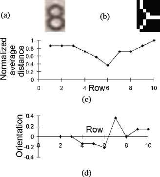
TS: (a) Character, (b) Skeleton of middle left zone, (c) Graph of
For the NPS intersection, and highlighting the a priori knowledge that we are in the presence of intersecting segments (see Fig. 9), the methodology considers that the segments are NPS if the
4.2. Global morphological characteristics vector
To optimize the relation between the number of data that describe the morphological characteristics and the quality of the information on them, a single row vector is generated that describes all the characteristics of the characters by concatenating the six equal size vectors that describe the characteristics of each zone. Table 2 details the possible values that the components of each of the six vectors of characteristics can have as a function of the geometric figure found.
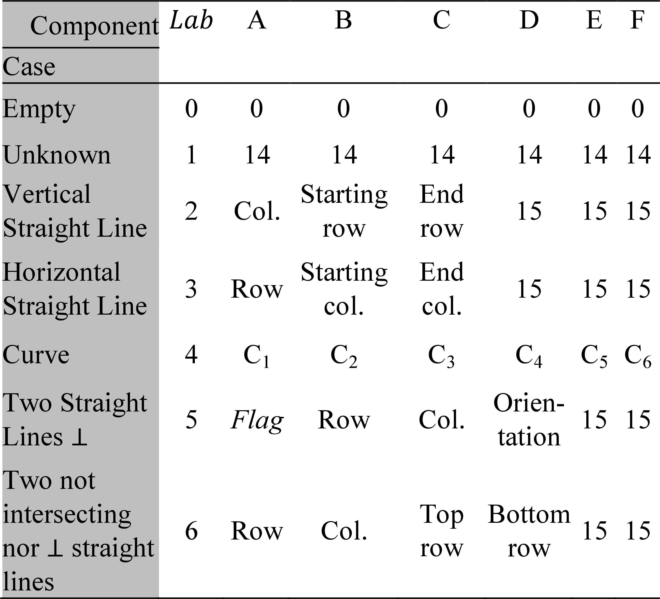
Vector of zone characteristics.
Emphasis is placed on the incorporation of the label component (Lab ∈ ℕ0 /Lab = 0, 1,..,6), which defines the type of figure found. On the other hand, in order to standardize the size of the six vectors of characteristics, flags are used that establish the types of perpendicular segments found, and tell the classification system that the zone has not been recognized (flag 14) or that the components do not have information (flag 15).
Finally, the ratio between the height and width of the character is added as the last morphological characteristic, which is duplicated in two new components to increase its weight in the classification process. This generates a Global Characteristics Vector (GCV) with 45 elements (see Fig. 18).
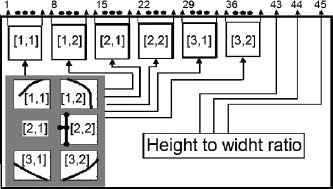
Characteristics global vector.
To validate the efficacy of the EMC a qualitative process based on the visual inspection of the results represented by an algorithm that “draws” the character from the extracted characteristics is developed. Three types of results are established that define the quality of the characteristics as a function of their visual similarity with the original image and the number of zones in which the system recognized the figure. They are:
- •
Correctly Extracted (CE): The figure and its dimensions are identified in the six zones.
- •
Irregularly Extracted (IE): The figure and its dimensions are identified in only five zones.
- •
Not Extracted (NE): Does not fulfill any of the above.
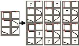
Fig. 19 shows graphic representations of extracted morphological characteristics, with the zones that were not identified indicated by “?”. Table 3a shows a quantitative analysis of the three qualitative variables defined for a total of 500 sample images.
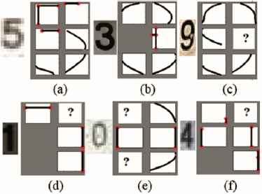
Representation of EMC: (a and b) CE, (c and d) IE, (e and f) NE.
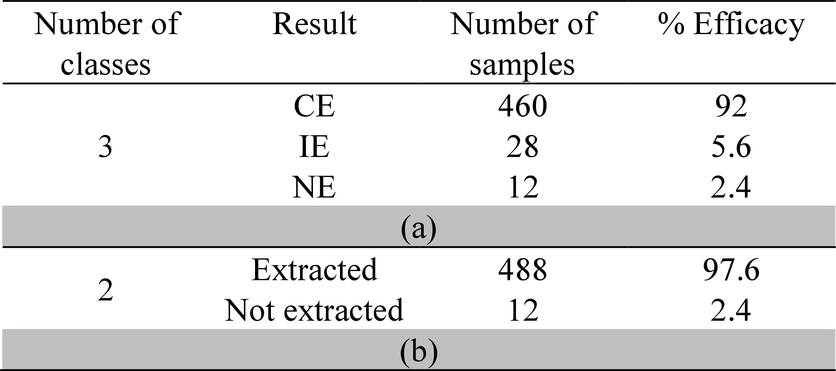
EMC results.
Since the designed OCR method considers a correct recognition of characters with at least five of its six zones well recognized, it is possible to reanalyze the efficacy as a function of its usefulness for the proposed classification system. The results of this analysis are shown in Table 3b, and they allow knowing beforehand the upper bound of global efficacy of the proposed tool as 97.6 %.
5. Classification of Global Vector of Morphological Characteristics Extracted for the OCR
OCR corresponds to a classification problem, i.e., each input vector X ∈ ℝ45 is assigned as belonging to one of the ten classes that represent the numerical characters.
The selected classification method is that of Support Vector Machines (SVM), and its selection was based on its efficacy recorded in the literature and on a laboratory test comparing the SVM and the Artificial Neural Networks (ANN) methods, which among the systems based on learning are also a verified effective strategy [12, 13] and used in OCR [14].
SVM is a dichotomous classification system that is important in not linearly separable cases and having an effective performance in OCR [15, 16].
SVMs basically map points from an input space of l elements to a space of characteristics of greater dimension, and finds in it a hyperplane that separates the input points into two classes and maximizes the selection margin m represented on the right side of Fig. 20 [15, 17].
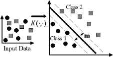
Input data not linearly separable taken to an SVM hyperplane.
The hyperplane sought by the SVM is given by
With respect to the Kernel, K(xi, xj), it calculates the dot product of the input vectors in the new characteristics space of greater dimension. It is necessary for the Kernels function to satisfy Mercer’s theorem, such as the grade d Kernel polynomial shown in (23):
5.1. Training data pre-processing
For the classifier to be capable of recognizing characters in which the morphological characteristics of five out of their six zones are correctly extracted, virtual training data is generated, sextuplicating GCVs obtained from CE numeric character images. With this purpose, six new GVCs are generated from each CE numeric character. Then, one of the six zones in each GCVs is alternately defined as non-identified, i.e. Lab = 1 (see Table 2). For example, Fig. 21 shows the graphic representation of the generation of “virtual training data”.
Graphic representation of “virtual training data”.
Considering the equilibrium among the problems related to the bias and to those of overparameterization and overlearning, the minimum value for training examples is obtained from the topology analysis of the ANN developed and determined by:
Although the generation of virtual training data increases the number of samples available for training ANN (see Table 4), the number of required samples calculated by means of equation (24) and equal to 9,440 is still not obtained. In order to solve this problem, the total number of samples (1,450) was septuplicated, obtaining a new value equal to 10,150.
| Character Type | Number of examples | Total |
|---|---|---|
| Correc. extracted | 20 for each character | 200 |
| Irreg. extracted | 5 for each character | 50 |
| Virtual data | 120 for each character | 1,200 |
| Total | 145 for each character | 1,450 |
| Septuplication total | 1015 for each character | 10,150 |
Training data.
5.2. Development of SVM
Considering the dichotomous nature of the SVM classification and the multiclass nature of the problem, a multiclass classification system was developed using the “multisvm” algorithm (MATLAB®), whose operation is based on the one against all methodology that is owned by Anand Mishra.
The generation and training of the ten different SVMs was carried out by means of the “svmtrain” function owned by MATLAB®, where the hyperplane was sought by the Sequential Minimal Optimization (SMO). Parameter C set at one, and the kernel used is a third degree polynomial, whose choice was based on the ease that it has to accommodate to curves. Table 5 shows indicators and parameters of the training that was carried out.
| C | Optimization method | % KKT violation | Kernel | R |
|---|---|---|---|---|
| 1 | SMO | 0 | 3rd degree polynomial (ec. 23) | 1 |
SVM training.
5.3. Development of ANN
The developed ANN corresponds to a feed-forward backpropagation of a hidden layer where the output is four bits that represent the recognized character in base 2. The main characteristics of the developed ANN are shown in Table 6.
| Layer | Input | Hidden | Output |
|---|---|---|---|
| Number of neurons | 45 | 20 | 4 |
| Activation function | --- | tanh | logsig |
Parameters of developed ANN.
An analysis of the results of “global vectors of characteristics” obtained in laboratory tests led to the conclusion that the ranges of values of the different components of the vector of characteristics always belong to the range of values −2 ≤ x ≤ 15 with x ∈ ℝ, which allowed reducing the range of input data of the ANN.
The training carried out corresponds to a supervised one with incremental weight updating. Table 7 shows the algorithms used for the training, which was carried out by means of the “train” function (Matlab®), where the main indicators of the training are illustrated in Table 8.
| Training stage | Algorithm used |
|---|---|
| Training | Levenberg-Mardquardt |
| Performance | Mean Squared Error |
Training algorithms used.
| Number of iterations | Performance | Gradient | Mu | R |
|---|---|---|---|---|
| 16 | 2.56 · 10−8 | 3.27 · 10−6 | 10−8 | 1 |
Results of the ANN training.
6. Results of the Proposed Tool
The validation was made with 500 data, equivalent to 76.9 % of the total data available for the development and validation of the tool. The classification by SVM of the 500 data is shown in Table 9, achieving a global efficacy equal to (95 +/- 3) % and a processing time close to 0.4 s, while the classification by ANN for the total data was equal to (92 +/- 4) %, with a processing time of 0.35 s.
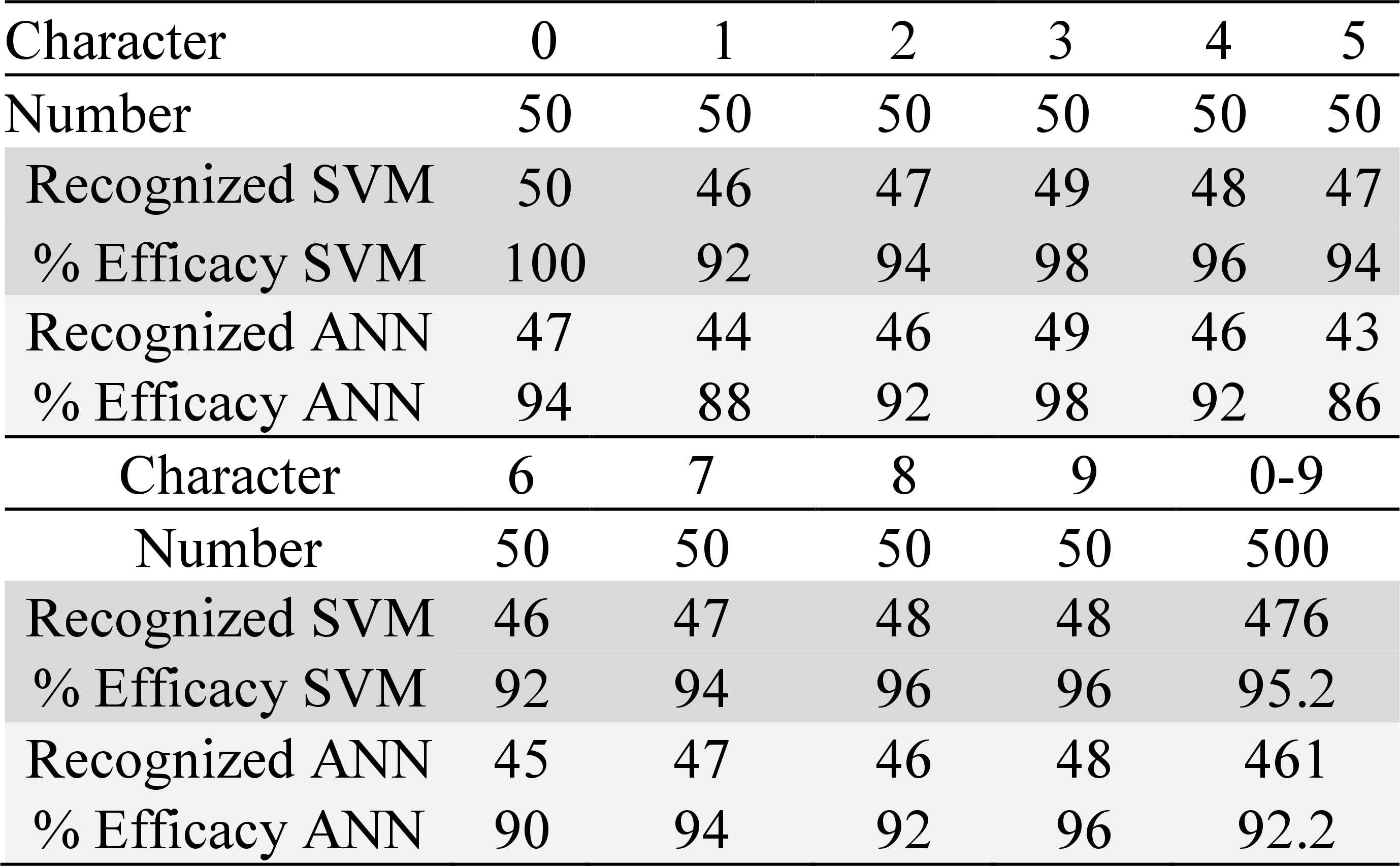
Results of SVM and ANN.
Fig. 22 shows illustrations of the global results of the developed tool using SVM, with the numbers in parentheses indicating the recognized character. Fig. 23 shows a comparison between the efficacy obtained by SVM and ANN for the classification of each character.
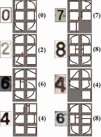
Results of classification with SVM.
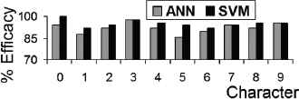
Comparison of efficacy.
6.1 Results comparison
The inexistence of specialized literature related to the recognition of previously segmented license plates must be noted. In this context, Table 10 shows a comparison of the method proposed for OCR with other methods, which was obtained from research on LPR.
| Method | Efficiency % | Advantage(s) | Disadvantage(s) | A | B |
|---|---|---|---|---|---|
| 1 | 95 %, for a total of 500 samples. | Stores pseudo- real morphology of the character. Binarization based on grouping pixels for obtaining images “containing” the characters produces results more independent from the specific position of the image’s zone to be processed. |
Long processing time. | Yes | 400 ms |
| 2 | 79.8 %, for a total of 214 samples. | The classification characteristics used allow for knowing the pseudo-real morphology of the character to a certain extent. | Binarization based on the use of threshold levels for obtaining images “containing” the characters produces results dependent on the specific position of the image’s zone to be processed. Only allows +/- 5° rotation of characters. | No | ND |
| 3 | 89 % (in LPR), for a total of 1,148 samples. | Low sensitivity to luminance changes in the image. | Binarization based on the use of threshold levels for obtaining images “containing” the characters produces results dependent on the specific position of the image’s zone to be processed. | No | 128 ms |
| 4 | 94 % (in LPR). | Low use of computing sources. | Binarization based on the use of threshold levels for obtaining images “containing” the characters produces results dependent on the specific position of the image’s zone to be processed. | No | ≈ 370 ms (in LPR) |
| 5 | 95.6 %, for a total of 322 samples. | Considering the character templates referred to the pseudo-analysis of connected components considerably improves the typical performance of the template comparison method. | Binarization based on the use of threshold levels for obtaining images “containing” the characters produces results dependent on the specific position of the image’s zone to be processed. | No | ND |
Comparison of methods for OCR, where: A = Does it store pseudo-real morphology of the character?; B = Execution time and ND = non-defined.
The compared methods are the following:
- 1.
Method proposed in this research.
- 2.
Method developed by Shidore, et al. [19]; based on the use of SVM for classifying the character features, which are composed of the number of transitions detected (binary images) by scanning lines that start from the character’s “mass center” and move towards its outer side.
- 3.
Method developed by Anagnostopoulos, et al. [2]; based on the use of a probabilistic neural network for classifying the character features, which are represented by data obtained through the analysis of components connected to zones of the image, in turn, determined by two concentric windows that scan the image.
- 4.
Method developed by Amir Hossein Ashtari, et al. [1]; based on a hybrid classification system composed of a decision-tree and SVM.
- 5.
Method developed by Rong and Yanping [4] based on a waterfall algorithm with two stages for template comparison.
The analysis of the method comparison for OCR shown in Table 10 allows us to suggest that:
- •
The proposed method exhibits a good numeric character recognition performance.
- •
The proposed method has a longer processing time than the other methods.
- •
The proposed method is unique in that, among the set of compared methods, allows for pseudo-really obtaining the morphology of the recognized character. This information may be used in further studies on IA.
- •
The problem concerning image binarization through the use of threshold levels, even when obtained by means of some optimization method, is partially solved in the proposed method.
7. Conclusions
The present restrictions of the LPR systems show that this an issue that is not fully solved.
The use of the morphology of the pseudo-real outline of the skeleton of the characters as classification characteristic allows a reduction of the restrictions in LPR, with processing times within the current documented range.
The use of images of vehicles for sale provided a semi-controlled scenario and new method of validation.
The interaction of K-Means and the Fuzzy system allowed the fine segmentation of the character, with an average efficacy of 99.2 % in spite of the poor quality of some images. The elimination of details, the skeletization and trimming of the image facilitated the later EMC.
The search for predefined figures in the six zones of the character, based mainly on the analysis of
Considering a geometric tolerance based on the greater visual importance of larger size objects allowed improving the recognition of straight lines in spite of their possible distortions.
The generation of virtual training data allowed the classification of characters in which only five of their zones show a correct EMC.
Comparison of results in the classification between the SVM and the ANN shows the better performance of the SVM.
There is a relation between the classification error of the characters “2”, “6” and “8” and the similarity of their extracted morphological characteristics, which would improve by adding a second activated classifier, if the character corresponds to one of those specified.
Finally, the tool developed for the recognition of numerical characters of license plates shows an efficacy of (95 +/- 3) % for a total of 500 samples obtained from semi-controlled scenarios, a processing time of approximately 0.4 s, and a relaxation of the restrictions.
Acknowledgements
This work has been supported by Proyectos Basales and the Vicerrectoría de Investigación, Desarrollo e Innovación (VRIDEI), Universidad de Santiago de Chile, Chile.
Footnotes
Visual similarity of form that the skeleton obtained with the “actual” outline of the character has.
References
Cite this article
TY  - JOUR
AU  - H. Olmí
AU  - C. Urrea
AU  - M. Jamett
PY  - 2017
DA  - 2017/01/01
TI  - Numeric Character Recognition System for Chilean License Plates in semicontrolled scenarios
JO  - International Journal of Computational Intelligence Systems
SP  - 405
EP  - 418
VL  - 10
IS  - 1
SN  - 1875-6883
UR  - https://doi.org/10.2991/ijcis.2017.10.1.28
DO  - 10.2991/ijcis.2017.10.1.28
ID  - Olmí2017
ER  -