
A New Approach for the 10.7-cm Solar Radio Flux Forecasting: Based on Empirical Mode Decomposition and LSTM
 , Liucun Zhu1, *, Hongbing Zhu1, Wei Chien3, Jiahai Liang3
- DOI
- 10.2991/ijcis.d.210602.001How to use a DOI?
- Keywords
- Solar radio flux; Time series forecasting; Empirical mode decomposition (EMD); LSTM
- Abstract
The daily 10.7-cm Solar Radio Flux (F10.7) data is a time series with highly volatile. The accurate prediction of F10.7 has a great significance in the fields of aerospace and meteorology. At present, the prediction of F10.7 is mainly carried out by linear models, nonlinear models, or a combination of the two. The combination model is a promising strategy, which attempts to benefit from the strength of both. This paper proposes an Empirical Mode Decomposition (EMD) -Long Short-Term Memory Neural Network (LSTMNN) hybrid method, which is assembled by a particular frame, namely EMD–LSTM. The original dataset of F10.7 is firstly processed by EMD and decomposed into a series of components with different frequency characteristics. Then the output values of EMD are respectively fed to a developed LSTM model to acquire the predicted values of each component. The final forecasting values are obtained after a procedure of information reconstruction. The evaluation is undertaken by some statistical evaluation indexes in the cases of 1-27 days ahead and different years. Experimental results show that the proposed method gives superior accuracy as compared with benchmark models, including other isolated algorithms and hybrid methods.
- Copyright
- © 2021 The Authors. Published by Atlantis Press B.V.
- Open Access
- This is an open access article distributed under the CC BY-NC 4.0 license (http://creativecommons.org/licenses/by-nc/4.0/).
1. INTRODUCTION
Accurate forecasting of F10.7 forecasting plays an important role in the fields of space weather and aerospace. For instance, the density of Earth's atmosphere can be driven by the variant F10.7 emitted from the Sun, which would disrupt the motion trajectory of objects in low earth orbit. Therefore, a short-to-medium term F10.7 forecasting is required to develop for the orbit parameters determination and collision warning before spacecraft launch mission [1]. However, the F10.7 daily values are characterized by high volatility and nonlinearity, and the relationship between F10.7 and the solar activity is close but not always constant, which makes the predicted behavior challenging [2,3]. Moreover, as the deterioration of the observational environment, the F10.7 time series contains some types of noise, which predicts F10.7 more difficult [4,5].
Some scholars attempt to predict the F10.7 by the linear model. Ref. [6] adopt a recursive linear autoregressive model, i.e., use the first n days to predict the next one day, and then the predicted value will be applied to the next prediction as to the input value of the model and so forth. Ref. [7] proposed a linear model to predict F10.7 of the following 1-45 days with the past 81 days' values. The experiment results showed that the correlation of prediction obtained by this method was between 0.85 (40-day ahead) and 0.99(1-day ahead), which is almost precisely compared to the traditional artificial neural network (ANN) models. On the other hand, the magnetic flux models were proposed by some literatures [8–12], which looked like promising approaches.
During the past two decades, With the spring up of machine learning technology, there has been an overwhelming interest in almost all fields applied by machine learning approaches, including time-series forecasting on energy consumption [13,14] and price index on international trade [15], etc. Ref. [16] demonstrates a feedforward neural network (FNN) for 1-day ahead forecasting. The data from 1978 to 1988 was chosen as the training set and the data in 1993 as the test set. The experimental results show that the increase of the hidden layers number does not play a decisive role in the prediction accuracy. Correspondingly, there is no significant correlation between them. Ref. [17] proposed the Support vector regression (SVR) for the short-term prediction of F10.7. This method considered a kernel-based learning algorithm to reduces the computational complexity in the training process. The results showed that this method can achieve accuracy close to the traditional FNN with fewer data. However, the paper suffers from insufficient sample size to cover the prediction under moderate level solar activity. Besides, the author has not been able to specify the reference model, which makes it impossible for us to know precisely where the prediction level is. Ref. [18] presented Back Propagation (BP) neural network algorithm to the F10.7 forecasting, which applied the previous 54 days as the input number of the neural network to predict the coming 1-3 days. The result is superior to the SVR method in short-term forecasting. Nevertheless, the study is limited by the poor performance in 2003 and 2004 when is the years of high solar activity. Recently, the Long Short-Term Memory (LSTM) model is also widely applied to time-series forecasting and acquired a superior effect [19,20].
Compared with other algorithms, the neural network has a stronger ability to approximate the nonlinear function. Nevertheless, as a stochastic training algorithm, its training effect is easily affected by the changes of the hyperparameters, such as the input number, the hidden layer number, the learning rate of optimizer [21,22]. Besides, the hyperparameters selection mainly relies on manual modulation since there is no mathematical formula to follow. To mitigate this negative impact, many scholars have recently tried to use a hybrid algorithm to improve prediction accuracy. Some scholars make a combination of optimization algorithms and ANNs. The hyperparameters are firstly fixed by optimization algorithms, such as genetic algorithm (GA) and particle swarm optimization (PSO), and then the data would be trained by the neural network [23–25]. The strategy above allows to improved the prediction accuracy to some extent. Nonetheless, its high computational complexity limits its application in practice. More recently, some scholars used the Empirical Mode Decomposition (EMD) to combine the ANN for solving the chaos time series problems. Ref. [26] developed a reliable method of bearing fault diagnosis based on EMD and ANN. The EMD was used to extract the features from vibration signals of rolling element bearings. Some intrinsic mode functions were selected and then trained by ANN to classify different bearing defects. Ref. [27] proposed an EMD-based FNN technique for wind speed forecasting. The results showed that the technique could improve the prediction accuracy of nonstationary and nonlinear time series compared with FNN. Ref. [28] designed the EMD coupled with autoregressive integrated moving average (ARIMA) for the hydrological time series forecasting. The annual runoff data was firstly preprocessed before through the ARIMA forecasting model, aiming at insight into the characteristics of original data. The results showed that their proposed model could significantly improve the forecasting effect of ARIMA. All the results mentioned above indicated that the EMD can effectively expose the regularity of the original time series, which allows reducing the chaotic characteristic. By pairing with ANNs, the EMD offers a significant enhancement in the field of time series prediction.
In this paper, a hybrid algorithm based on EMD and LSTM neural network is proposed for the 1-27 days forecasting of F10.7. First, the dataset of F10.7 is separated into a series of IMFs with specific frequency information by EMD. Subsequently, the output value of EMD is trained in LSTM as the input value of the neural network. Finally, the output values of LSTM, which are the predicted values of each IMF and residual, are reconstructed to the final F10.7's forecasting value. The experimental results would be compared with BP, LSTM and EMD–BP.
This paper is organized as follows: Section 2 introduces the LSTM neural network and EMD–LSTM method proposed in this paper. Section 3 introduces the F10.7 dataset partition, evaluation indicators and hyperparameters selection. Section 4 analyzes the forecasting effect in detail. At the end of the article, we will make a summary and put forward the direction for future work.
2. PROPOSED METHODS
2.1. Conventional LSTM
LSTM is an excellent variant model of Recurrent Neural Network (RNN) proposed by Hochreiter and Schmidhuber [29]. As a result of the solution of vanishing gradients and exploding gradients, the LSTM network is well-suited to handling the time series problems with long duration [30]. The hidden layer of LSTM has a particular unit called the cell, which contains three different types of the gate that can control the flow of information in cells and neural networks. These components are the core part of information memory, and their internal structure is shown in Figure 1. Similar to RNN, LSTM belongs to the feedback neural network, of which the training process is realized by the forward algorithm and backpropagation through time (BPTT) algorithm. The forward algorithm is shown in the following formula [31,32]:
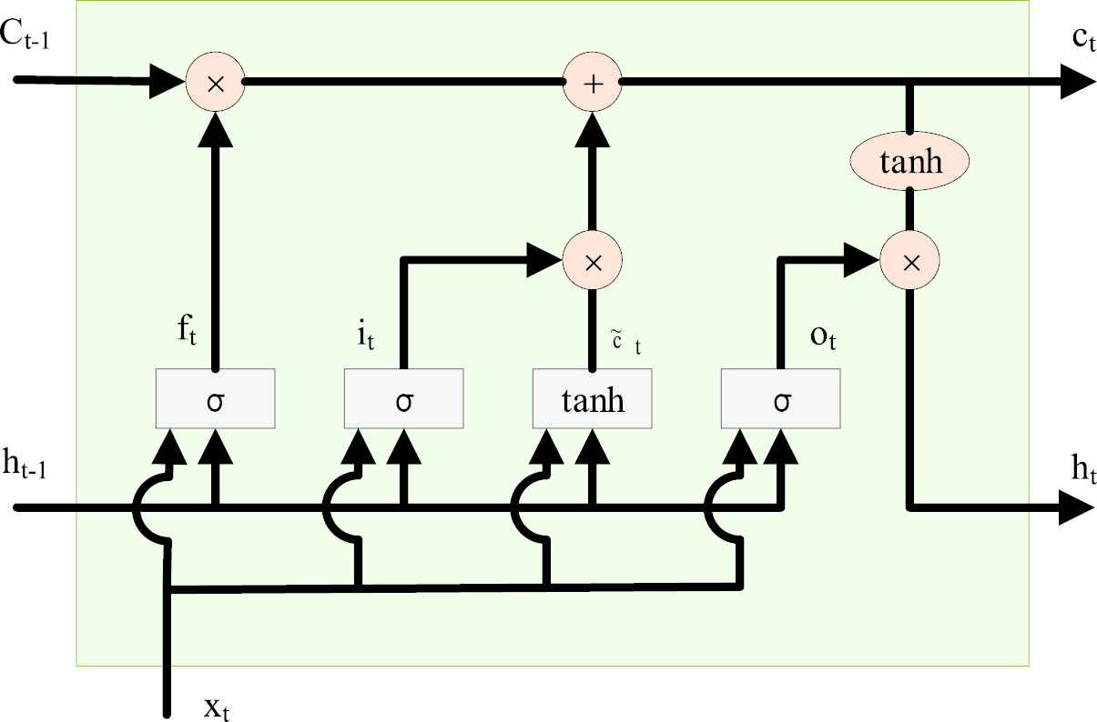
Structure of cell in Long Short-Term Memory (LSTM).
Where
The value of
The training process of LSTM model can be roughly divided into four steps. Step1: calculating the output value of LSTM according to formula (1) – (6); Step2: According to the structures on time and network, calculate the error terms of each LSTM cell in reverse on two propagation directions; Step3: According to the terms of error, calculate the gradient of each weight; Step4: update the weight by the gradient-based optimization algorithm.
2.2. EMD–LSTM Method
The EMD is a signal decomposition method based on local characteristics of signals proposed by Ref. [35]. It is suitable for nonlinear and nonstationary signal analysis. In the EMD–LSTM model, the EMD decomposes the original signal step by step and generates a series of data sequences called IMF. Further, IMFs as input are trained by the LSTM model in order to acquire the predicted values of IMF. In the end, the predicted values of each IMFs are accumulated to get the final predicted values. The schematic diagram of EMD–LSTM is shown in Figure 2. This sifting process is described as follows [36,37]:
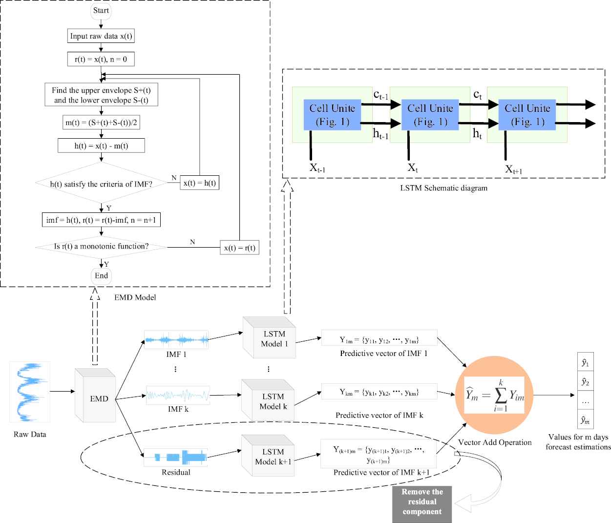
Empirical Mode Decomposition–Long Short-Term Memory (EMD–LSTM) schematic diagram.
Step1: Recognize all the local extremum values from the original signal
Step2: Find the IMF item
Step3: If
Where
Step4: The renewal of the residual. With
Step5: Consider
Step6: For predicting the following m days, the IMFs will be treated as input data and be trained separately by LSTM model, aiming to obtain the predicted values of correspondent IMF
Step7: The forecasting values of each IMF
Computational complexity. The neural network we used in the proposed method is a typical 3-layer LSTM net, which contains an input layer, a recurrent LSTM layer, and an output layer. The input layer is connected to the LSTM layer. The LSTM layer consists of a single cell, which is maintained by an input gate, a forget gate, an output gate and a candidate gate. The LSTM layer is a recursive structure and is therefore connected directly from the cell output unite to the cell input unit. The cell out unite is finally connected to the output layer of network [31]. The total number of parameters
Where
3. DATA ANALYSIS
3.1. Data Source
The dataset we selected is the daily values of F10.7 from the Center for Space Standards and Innovation (http://www.celestrak.com/SpaceData/SW-All.txt). All of the values are adjusted to 1 AU, which is the average distance between the Earth and Sun. Otherwise, the observations cannot be measured by the uniform standard, which will further increase the complexity of the time series. The spectrum of dataset covers from 1980 to 2014, giving a total of 12,784 observations, and about 65.7% of the total values from 1980 to 2002 serve as the training set of the LSTM neural network. The remaining contained 4,383 values from 2003 to 2014 serves as the test set. The partition information of data is shown in Table 1.
| Description | Numbers | Proportion (%) |
|---|---|---|
| All samples | 12,784 | 100 |
| Training samples | 8,401 | 65.7 |
| Test samples | 4,383 | 34.3 |
Description of data set.
3.2. Evaluation Methods
To objectively evaluate the performance of the methodology involved in this paper, five statistical evaluation indexes are used: Mean Absolute Percentage Error (MAPE), Root Mean Square Error (RMSE), Normalized Mean Square Error (NMSE), correlation coefficient (R) and spearman correlation coefficient (
| Metrics | Calculation | Evaluation Criteria |
|---|---|---|
| MAPE | The closer to 0, the better | |
| RMSE | The closer to 0, the better | |
| NMSE | The closer to 0, the better | |
| R | The closer to 1, the better | |
| The closer to 1, the better |
MAPE, Mean Absolute Percentage Error; NMSE, Normalized Mean Square Error; RMSE, Root Mean Square Error.
Evaluation indices.
Where n is the number of samples,
3.3. IMF (Intrinsic Mode Functions) Data Analysis
The F10.7 dataset used in this paper is processed by EMD and generates eleven IMFs and the sole residual. The decomposition results are shown in Figures 3 and 4. IMF1 and IMF2 show as chaotic signals in Figure 3 and their regularity can not be recognized. Its instantaneous frequency in Figure 4 shows the frequency with a high change rate which is interwoven by the various frequency signals and contains a large amount of noise. The instantaneous frequency of IMF3-IMF8 show sharp decreases in frequency fluctuations, and also ascending frequency stabilities. IMF9-IMF11 show increasing monotonicity tends, which indicates enlarged predictability. Among them, IMF9 reflects the changing trend in the medium-term, whereas IMF11 reflects the changing trend in the long-term.
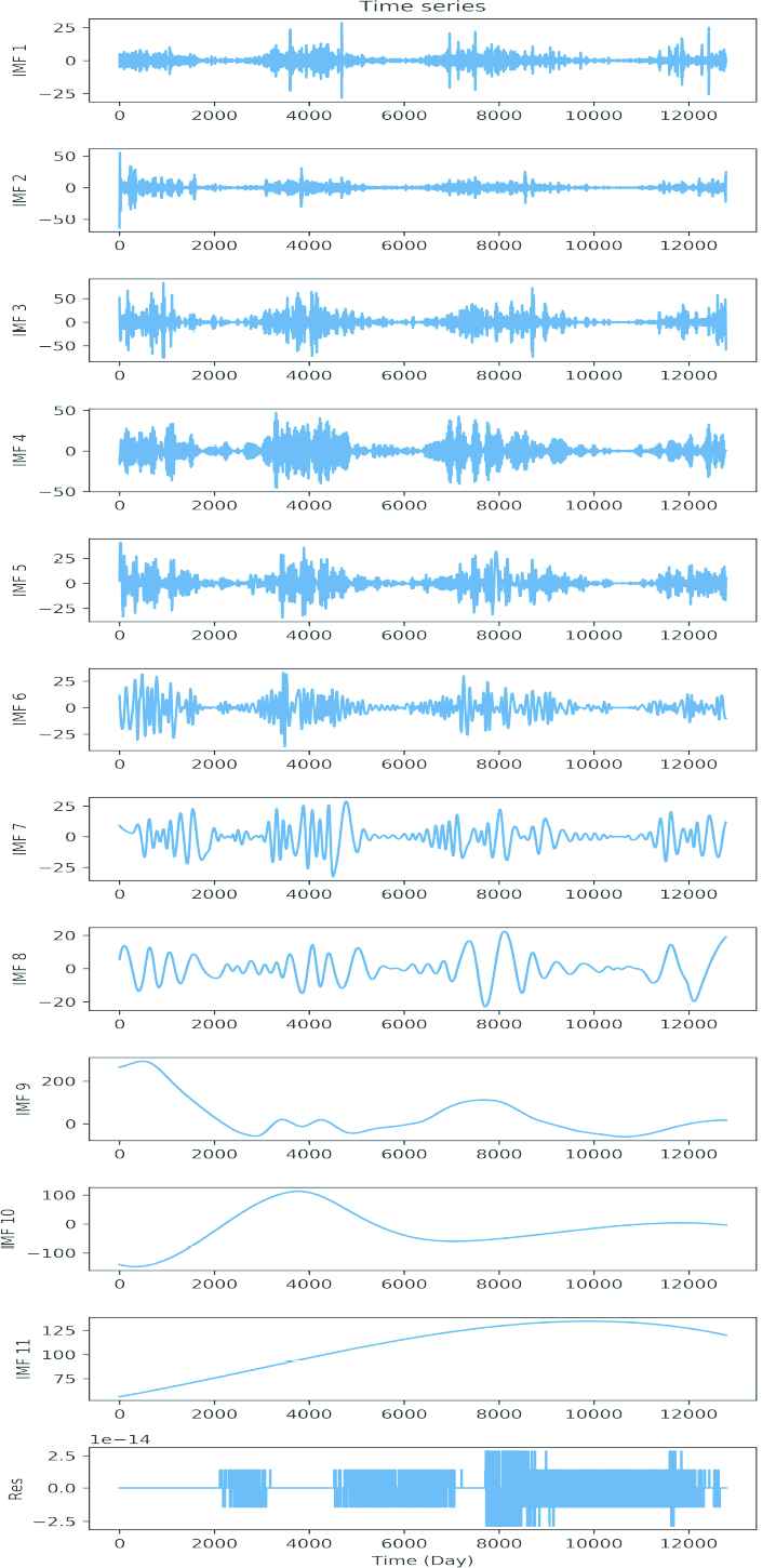
Curve of Empirical Mode Decomposition's (EMD's) components, showing 11 out of 11 IMFs and the residual.
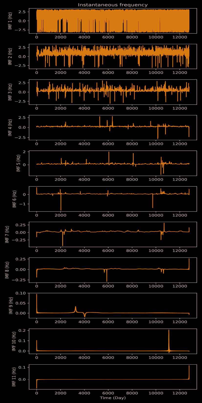
Instantaneous frequency of each scale of Empirical Mode Decomposition (EMD), showing 11 out of 11 IMFs.
In this experiment, the final result does not include the residuals. That is because, after analysis of the IMF curves from Figure 3, we found the residual carried an extremely small amount of information (with the order of
3.4. Parameters Selection of LSTM
The LSTM model used in this paper is a typical 3-layer neural network. According to the empirical formula [39], the number of hidden neurons was set to 12. The Adam optimizer was selected because of its high computational efficiency [40], which also maintained the stable training effect in low signal-to-noise ratio signals. The iteration is set to be 500. Also, we evaluate the predictive effect of the nodes number in the input layer, the results are shown in Figure 5. When the number of input nodes is 1, the prediction errors in all 1-27 days were significantly higher than those in others. When the number of input nodes was greater than 1, the prediction effect was approximately kept at the same level. Additionally, under the same number of input nodes, the prediction error went up with the rise of prediction days, ranging from 2% (1-day ahead) to 6.5% (27-day ahead). Therefore, in this experiment, we set the number of inputs to 2, which used the past two days to predict the following days.
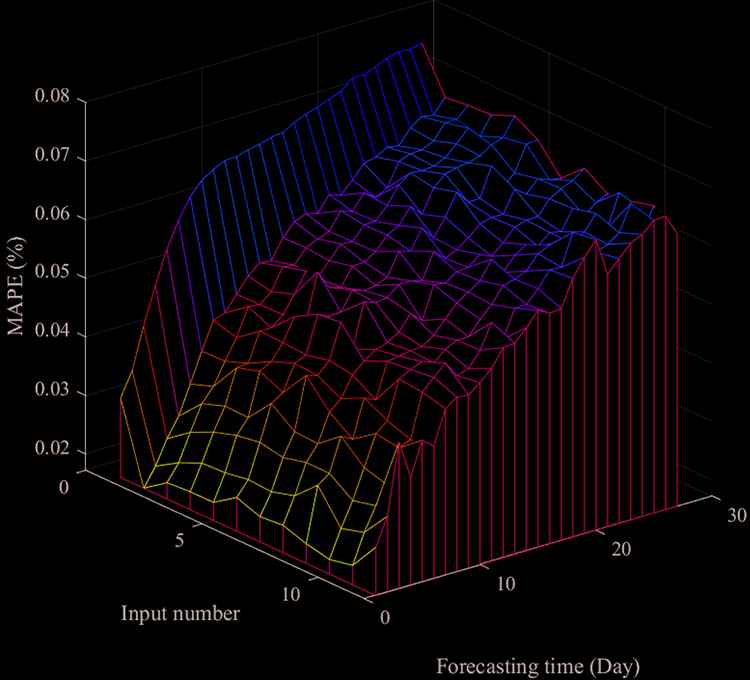
Distribution of Mean Absolute Percentage Error (MAPE) among different nodes number in input layer and forecast days.
4. EXPERIMENTAL RESULTS AND DISCUSSION
4.1. The Correlation Coefficient Analysis of Components
The forecasting correlation of each scale was shown in Figure 6. The IMF1 has the lowest correlation, ranging from 0.01 (27-day ahead) to 0.05 (1-day ahead), which indicated that the prediction model has a weak prediction effect on IMF1. The correlation between IMF2 and IMF3 has a surge increase but is still situated at a low level. slowed down. The correlation between IMF4 and IMF6 was higher than 0.9900, showing good results. Nonetheless, there were still some intervals below 0.9000 in the medium-term. IMF7-IMF11 could be treat as almost the same level of correlation, which was at an extremely high level. The correlation of IMF11 in 1-27 days is 1, which indicated the full predictability of the trend. IMF1-IMF3 have a high instability, which made the prediction model unserviceable. With the growth of the IMF scales, the prediction accuracy significantly rises. Overall, under the same forecast days, the deeper the scales of EMD, the larger the correlation will obtain. Additionally, on the same scale, the correlation decreases with the extension of forecast days.
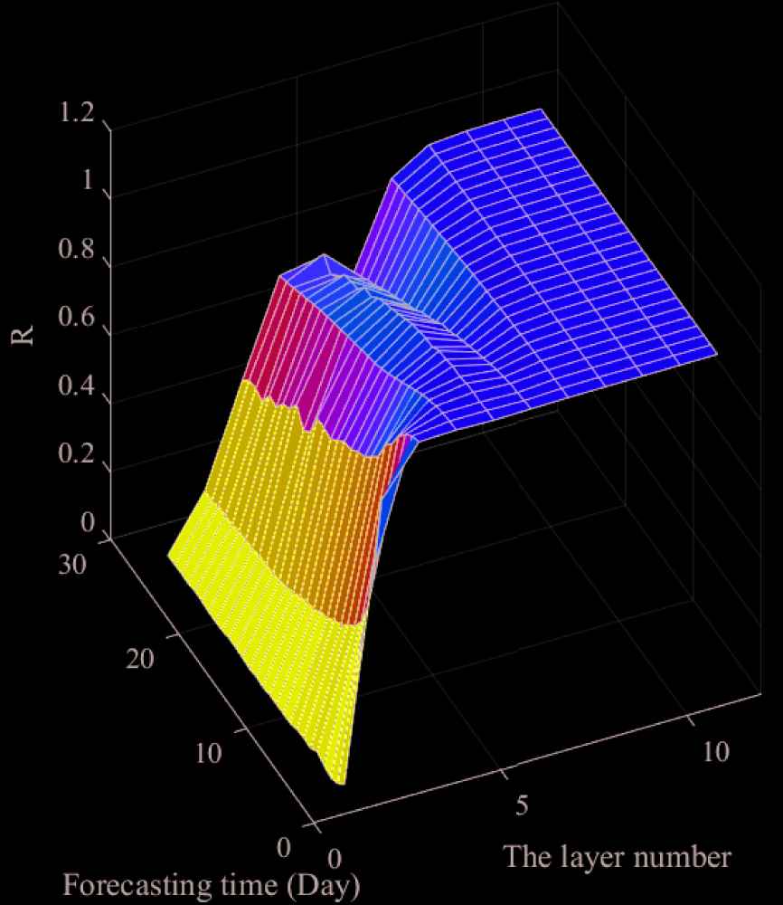
Distribution of correlation coefficient among different scale of Empirical Mode Decomposition (EMD) in different forecasting days.
4.2. The Performance Analysis in Different Solar Activity Years
We compared the yearly MAPE of 3-day ahead in 2003-2012, which contained the years in high, medium and low solar activity. The results were shown in Figure 7. The maximum value of MPAE was obtained in the peak year of solar activity in 2003, with a value of 4.28%. From 2003 to 2008, the MAPE showed a continuous downward trend. Between 2009 and 2012, the MAPE showed a rebound trend. The results above demonstrated that the MAPE value has a high positive correlation with the solar activity level, which is consistent with the results in the relevant literatures [17,18].
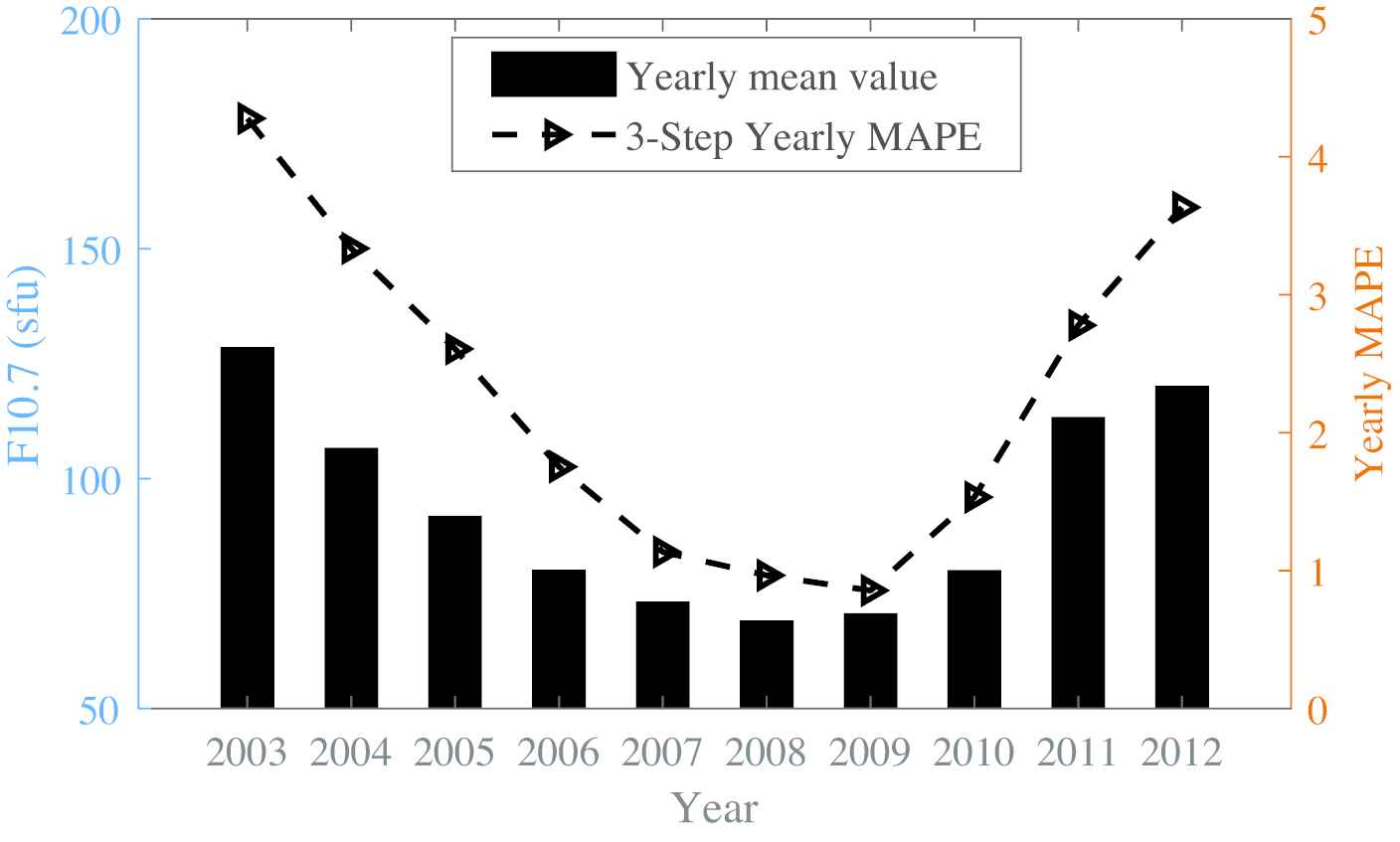
Distribution of yearly Mean Absolute Percentage Error (MAPE) in different years.
Furthermore, some conventional models were compared by our method. Ref. [17] used an SVR model to predict the next three days. The data from 2002 to 2006 used as the training set, and the data from 2003 to 2006 used as the test set. Ref. [18] used a typical three-layer BP model for the F10.7 forecasting. The maximum number of epoch set to be 100. That model used the past 54 days as the input to predict the following 3 days. The comparative results are shown in Table 3. In the years of high solar activity (in 2003), the average MAPE of EMD–LSTM is 3.28% in 1-3 days forecasting, which has a decrease of 56.3% and 43.9% compared with SVR and BP respectively. The values of NMSE and R are also optimum. In the years of moderate solar activity (in 2006), MAPE has a decrease of 58.6% and 40.4% compared with SVR and BP, the metrics NMSE and R were also outperformed the other three algorithms. In the years of low solar activity (in 2009), MAPE has an advantage of 71.5% and 53.2% over SVR and BP. The value RMSE is also significantly better than the other two algorithms under all conditions. For indicator
| Forecast Day | Year | MAPE (%) |
NMSE |
R |
||||||
|---|---|---|---|---|---|---|---|---|---|---|
| SVR | BP | EMD–LSTM | SVR | BP | EMD–LSTM | SVR | BP | EMD–LSTM | ||
| 1 | 2003 | 5.56 | 3.73 | 2.35 | 0.18 | 0.12 | 0.02 | 0.9956 | 0.9988 | 0.9995 |
| 2006 | 2.71 | 2.16 | 1.27 | 0.15 | 0.10 | 0.05 | 0.9993 | 0.9994 | 0.9998 | |
| 2009 | 1.71 | 1.08 | 0.59 | 0.12 | 0.08 | 0.01 | 0.9990 | 0.9994 | 1.0000 | |
| 2 | 2003 | 7.62 | 5.69 | 3.22 | 0.27 | 0.09 | 0.05 | 0.9933 | 0.9969 | 0.9989 |
| 2006 | 3.6 | 2.58 | 1.47 | 0.28 | 0.12 | 0.06 | 0.9988 | 0.9992 | 0.9998 | |
| 2009 | 2.96 | 1.77 | 0.77 | 0.19 | 0.10 | 0.02 | 0.9980 | 0.9991 | 0.9999 | |
| 3 | 2003 | 9.32 | 8.15 | 4.28 | 0.46 | 0.15 | 0.07 | 0.9886 | 0.9937 | 0.9983 |
| 2006 | 4.48 | 2.79 | 1.75 | 0.42 | 0.15 | 0.08 | 0.9982 | 0.9990 | 0.9997 | |
| 2009 | 3.11 | 1.91 | 0.86 | 0.30 | 0.20 | 0.02 | 0.9968 | 0.9983 | 0.9999 | |
BP, Back Propagation; EMD–LSTM, Empirical Mode Decomposition–Long Short-Term Memory; MAPE, Mean Absolute Percentage Error; NMSE, Normalized Mean Square Error; SVR, support vector regression.
Short-term comparison of yearly MAPE, NMSE and R in different solar activity years.
In the end, our method was also compared to the Ref. [41] models and the SWPC (Space Weather Prediction Center) model, used with the indicator
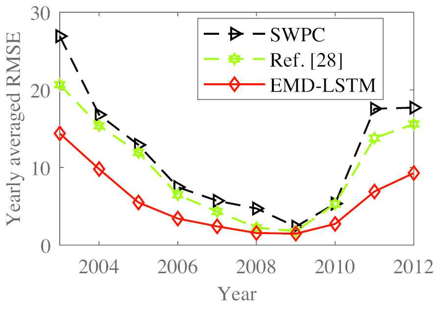
Comparison of yearly average Root Mean Square Error (RMSE) between SWPC, Ref. [28] and Empirical Mode Decomposition–Long Short-Term Memory (EMD–LSTM).
4.3. The Performance Analysis of Multistep Prediction
Figure 9 and Table 4 showed the performance comparison between BP, LSTM, EMD–BP and our method in 1-27 days forecasting. The MAPE has sharply grown in 1-8 forecast days. The MAPE of EMD–LSTM has an average value of 2.07% for 1-3 days forecasting, which has a decline of 43.0%, 37.4% and 21.2% compared with BP, LSTM and EMD–BP. The MAPE of ours has a global value of 5%, which has an improvement of 38.3%, 26.0% and 18.4% than of the above algorithms respectively. The RMSE and
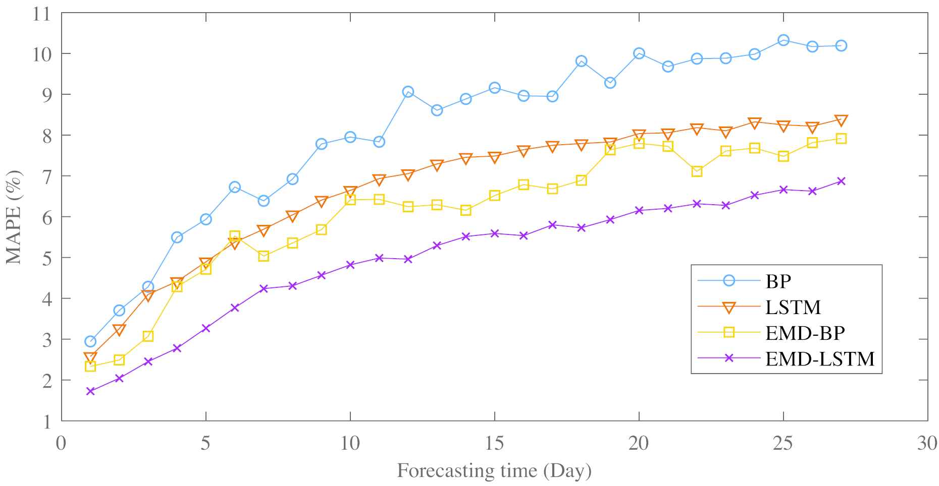
Comparison of Mean Absolute PercentageError (MAPE) between in 1-27 forecast days.
| Forecast Day | MAPE (%) |
RMSE |
||||||||||
|---|---|---|---|---|---|---|---|---|---|---|---|---|
| BP | LSTM | EMD–BP | Ours | BP | LSTM | EMD–BP | Ours | BP | LSTM | EMD–BP | Ours | |
| 1 | 2.94 | 2.58 | 2.33 | 1.73 | 5.48 | 4.94 | 4.26 | 3.51 | 0.99 | 0.99 | 0.99 | 0.99 |
| 2 | 3.70 | 3.26 | 2.49 | 2.04 | 6.95 | 5.99 | 4.37 | 3.93 | 0.98 | 0.98 | 0.99 | 0.99 |
| 3 | 4.28 | 4.10 | 3.07 | 2.45 | 7.73 | 7.27 | 5.48 | 4.58 | 0.97 | 0.98 | 0.98 | 0.99 |
| 4 | 5.50 | 4.41 | 4.29 | 2.78 | 9.25 | 8.21 | 7.66 | 5.26 | 0.97 | 0.97 | 0.98 | 0.98 |
| 5 | 5.94 | 4.89 | 4.71 | 3.27 | 10.88 | 9.33 | 7.32 | 6.19 | 0.96 | 0.97 | 0.97 | 0.98 |
| 6 | 6.73 | 5.38 | 5.31 | 3.77 | 11.76 | 10.10 | 9.00 | 6.77 | 0.95 | 0.96 | 0.97 | 0.98 |
| 7 | 6.39 | 5.69 | 5.04 | 4.24 | 11.94 | 11.05 | 8.39 | 7.57 | 0.95 | 0.96 | 0.97 | 0.98 |
| 8 | 6.92 | 6.05 | 5.36 | 4.31 | 12.87 | 11.66 | 9.47 | 7.92 | 0.95 | 0.95 | 0.97 | 0.97 |
| 9 | 7.78 | 6.41 | 5.68 | 4.57 | 13.17 | 12.21 | 9.95 | 8.33 | 0.94 | 0.95 | 0.96 | 0.97 |
| 10 | 7.95 | 6.65 | 6.41 | 4.82 | 14.46 | 12.49 | 11.72 | 8.61 | 0.92 | 0.94 | 0.95 | 0.97 |
| 11 | 7.83 | 6.93 | 6.42 | 4.99 | 13.79 | 13.06 | 11.70 | 8.88 | 0.93 | 0.94 | 0.95 | 0.97 |
| 12 | 9.06 | 7.06 | 6.25 | 4.96 | 14.71 | 13.49 | 11.02 | 9.03 | 0.90 | 0.93 | 0.95 | 0.97 |
| 13 | 8.61 | 7.29 | 6.29 | 5.29 | 15.09 | 13.61 | 11.22 | 9.36 | 0.92 | 0.93 | 0.95 | 0.97 |
| 14 | 8.88 | 7.46 | 6.16 | 5.51 | 15.01 | 13.89 | 11.15 | 9.66 | 0.91 | 0.93 | 0.95 | 0.96 |
| 15 | 9.16 | 7.49 | 6.52 | 5.59 | 15.56 | 14.10 | 11.88 | 9.76 | 0.90 | 0.93 | 0.95 | 0.96 |
| 16 | 8.96 | 7.64 | 6.79 | 5.54 | 16.20 | 14.18 | 11.98 | 9.84 | 0.90 | 0.93 | 0.95 | 0.96 |
| 17 | 8.95 | 7.75 | 6.68 | 5.80 | 15.78 | 14.38 | 12.48 | 10.36 | 0.91 | 0.92 | 0.95 | 0.96 |
| 18 | 9.81 | 7.79 | 6.89 | 5.73 | 16.87 | 14.47 | 12.37 | 10.54 | 0.89 | 0.92 | 0.94 | 0.96 |
| 19 | 9.28 | 7.83 | 7.64 | 5.93 | 15.61 | 14.59 | 12.64 | 10.49 | 0.91 | 0.92 | 0.94 | 0.96 |
| 20 | 10.00 | 8.04 | 7.80 | 6.15 | 15.41 | 14.70 | 12.96 | 10.85 | 0.91 | 0.92 | 0.94 | 0.96 |
| 21 | 9.68 | 8.06 | 7.72 | 6.20 | 16.50 | 14.86 | 12.98 | 11.02 | 0.90 | 0.92 | 0.94 | 0.96 |
| 22 | 9.87 | 8.18 | 7.11 | 6.32 | 16.51 | 14.83 | 12.47 | 11.28 | 0.90 | 0.92 | 0.94 | 0.96 |
| 23 | 9.88 | 8.10 | 7.61 | 6.28 | 16.30 | 14.98 | 12.90 | 11.35 | 0.91 | 0.92 | 0.94 | 0.96 |
| 24 | 9.98 | 8.32 | 7.68 | 6.53 | 16.84 | 15.03 | 13.28 | 11.70 | 0.90 | 0.91 | 0.94 | 0.95 |
| 25 | 10.33 | 8.25 | 7.48 | 6.66 | 17.61 | 15.15 | 12.25 | 11.79 | 0.89 | 0.91 | 0.94 | 0.95 |
| 26 | 10.17 | 8.22 | 7.81 | 6.63 | 17.97 | 15.06 | 13.24 | 11.83 | 0.89 | 0.91 | 0.93 | 0.95 |
| 27 | 10.19 | 8.39 | 7.92 | 6.87 | 17.16 | 15.14 | 13.44 | 12.10 | 0.89 | 0.91 | 0.93 | 0.95 |
BP, Back Propagation; EMD, Empirical Mode Decomposition; LSTM, Long Short-Term Memory; MAPE, Mean Absolute Percentage Error; RMSE, Root Mean Square Error; SVR, support vector regression.
Comparison of performance between BP, LSTM, EMD–BP and EMD–LSTM by multistep forecast.
Our method also compared with the linear models proposed by Ref. [1] and the transport model proposed by Ref. [11] under certain conditions, shown in Table 5. The values MAPE and RMSE of our method have a significant advantage with the other three algorithms in 1-day forecasting, and these advantages would be further extended in 3-day forecasting. The results of the three types of correlation parameters indicated that our method is better than the three algorithms.
| Forecast Day | Model | Spearman Coefficients | MAPE (%) | RMSE | Pearson Coefficients | R |
|---|---|---|---|---|---|---|
| 1 | Y | 0.98 | 3.38 | 5.56 | 0.98 | No provide |
| CH-MF | No provide | 3.5α | 3.7α | No provide | 0.9989 | |
| EMD–LSTM | 1 | 1.73 | 3.51 | 0.99 | 0.9994 | |
| 3 | Y | 0.98 | 4.12 | 6.13 | 0.97 | No provide |
| CH-MF | No provide | 6.1α | 7.3α | No provide | 0.9976 | |
| EMD–LSTM | 0.99 | 2.45 | 4.58 | 0.99 | 0.999 |
EMD, Empirical Mode Decomposition; LSTM, Long Short-Term Memory; MAPE, Mean Absolute Percentage Error; RMSE, Root Mean Square Error.
α means an approximate value, acquiring from the figures of corresponding reference literature.
Comparison between the observed and forecast values using the CH-MF and Y models.
4.4. The Analysis of the Fitting Effect
Figure 10 shows the fitting effect in 10-day advance forecasting in 2003 and 2008. On the whole, the fitting curve of the BP and EMD–BP model has an obvious deviation from the observed curve. The LSTM and EMD–LSTM model have a similar visual effect on the fitting curves, which can predict almost all the trends of F10.7 correctly. However, the prediction curve of EMD–LSTM model is smoother, and the fitting deviation at the extreme points is better than that of the LSTM model.
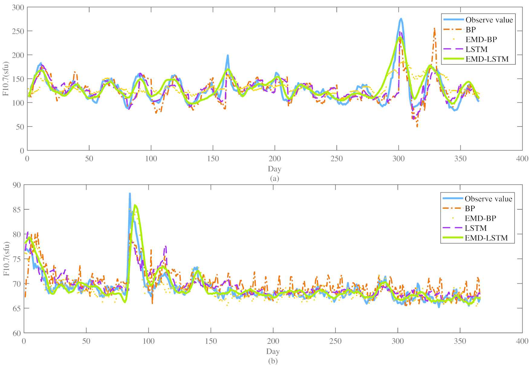
Fitting curve of forecasting. (a) Ten-step ahead forecasting in 2003. (b) Ten-step ahead forecasting in 2008.
According to analyze the fitting curve, we find the fitting error mainly comes from the local extreme points of the observe curves (i.e., around the 160th and 300th days in 2003 and the 90th and 120th days in 2008) which has a small proportion in the entire period. Therefore, as the imbalanced data, the features of local extreme points are always hard to be learning by Machine learning algorithms, which leads to the corresponding increase in forecast deviations in high solar activities.
5. CONCLUSION
The common F10.7 prediction models based on machine learning directly use the raw data as input, which leads to insufficient results. The reason for causing this problem may be that the neural network is not capable of extracting features from highly fluctuating original data. To overcome that problem, in this paper, a hybrid model EMD–LSTM is proposed to predict the F10.7 values. The raw F10.7 data is primarily treated by EMD and then breaks down into a series of IMFs and the residual, purposing to extract the features of frequency and reduce the complexity of the original signal. The independent LSTM models are then separately processed. The IMFs to acquire the predicted scale values of EMD. Finally, the predicted values of IMFs are synthesized to obtain the final forecast values. The experimental results demonstrate that our proposed method performs the best in all the testing cases.
We summarized the reasons that our method has impressive performance in short and medium-term prediction accuracy of F10.7 as follows: (1) EMD provides the ability to purify the features of the raw F10.7 signals, which will be beneficial to the further feature learning by the LSTM algorithm. (2) Compared with other machine learning algorithms, LSTM is more suitable for the scenarios of F10.7 prediction because of its memory characteristics.
Nonetheless, in high solar activity, the predicted deviation of our method is still relatively higher than that of low and medium solar activity. In future work, we will focus on exploring models to further improve the prediction accuracy of F10.7, such as finding a more suitable combination of noise reduction technology and neural network.
CONFLICT OF INTEREST
The authors declare no conflict of interest.
AUTHORS' CONTRIBUTIONS
All authors contributed to the work. All authors read and approved the final manuscript.
ACKNOWLEDGEMENTS
This research is supported by Special Fund for Bagui Scholars of the Guangxi Zhuang Autonomous Region and The Basic Ability Enhancement Program for Young and Middle-aged Teachers of Guangxi (Contract NO.2020KY10018).
REFERENCES
Cite this article
TY  - JOUR
AU  - Junqi Luo
AU  - Liucun Zhu
AU  - Hongbing Zhu
AU  - Wei Chien
AU  - Jiahai Liang
PY  - 2021
DA  - 2021/06/11
TI  - A New Approach for the 10.7-cm Solar Radio Flux Forecasting: Based on Empirical Mode Decomposition and LSTM
JO  - International Journal of Computational Intelligence Systems
SP  - 1742
EP  - 1752
VL  - 14
IS  - 1
SN  - 1875-6883
UR  - https://doi.org/10.2991/ijcis.d.210602.001
DO  - 10.2991/ijcis.d.210602.001
ID  - Luo2021
ER  -