
Arterial reservoir pressure, subservient to the McDonald lecture, Artery 13
- DOI
- 10.1016/j.artres.2013.10.391How to use a DOI?
- Keywords
- Arterial mechanics; Waves; Reservoir pressure
- Abstract
It is commonly assumed that pressure and flow in the arteries are purely the result of forward and backward travelling waves. We will show that various observations of arterial behaviour are difficult to explain using this assumption. In particular we will look at what happens to arterial pressure under different conditions: during ectopic beats, in experimental studies of pressure and flow when the aorta is totally occluded at different locations, in a computational study of the input impedances of randomly generated networks of arteries and when pressure and velocity are measured at different distances along the aorta.
We show that all of these observations can be explained using wave intensity analysis. We further show that this analysis suggests that it is useful to separate arterial pressure into a reservoir pressure that accounts for the overall compliance of the arterial system and an excess pressure that is determined by local conditions. Evidence has accumulated in the decade since the introduction of the reservoir-wave hypothesis that the reservoir/excess pressure separation can be useful in interpreting the results of vasoactive drugs on cardiovascular performance and that parameters based on the reservoir/excess pressure are significant predictors of cardiovascular events.
The important question that remains to be answered is the usefulness of the concept in the interpretation, physiologically and clinically, of the complex behaviour of the cardiovascular system. We conclude that the evidence suggests that it is a worthwhile topic for future research.
- Copyright
- © 2013 Association for Research into Arterial Structure and Physiology. Published by Elsevier B.V. All rights reserved.
- Open Access
- This is an open access article distributed under the CC BY-NC license.
Introduction
The title and the spirit of this paper are borrowed from Thomas Young’s paper Hydraulic investigations, subservient to an intended Croonian lecture on the motion of blood34 which is a collection of thoughts relevant to his Croonian lecture to the Royal Society in 1809 which, in turn, prepared the ground for the study of the mechanics of blood flow in arteries.35 One hundred and fifty years later, Donald McDonald wrote Blood Flow in Arteries12 which provided the foundations for modern hemodynamics; a field that has flourished in the past fifty years. The greatly expanded 2nd edition was a constant guide in my early years in arterial mechanics.13 The success and importance of his book is measured by the recent publication of the 6th edition.14 I am deeply honoured to have been invited to give the McDonald lecture at Artery 13 entitled Waves, Reservoirs and Arteries and this paper is a collection of thoughts relevant to that lecture.
The first question we need to address is ‘Why are we still holding Artery meetings?’. Arterial flow has been studied for centuries and the list of scientists who have contributed is long and distinguished, yet there are still many open questions about the physiology and pathology of the cardiovascular system. In the following, I will argue that some of these outstanding questions arise from the application of theoretical models that are too simplistic to accommodate the mechanical complexity of the arterial system (ignoring the vastly greater complexities at the cellular and molecular level). In support of this argument I will discuss four observations of arterial behaviour where our current understanding is not complete.
Before discussing these observations, however, it is necessary to define what is meant by ‘wave’; a word that has different meanings to different people. I will use the following definitions to avoid confusion (see Fig. 1):
- 1)
‘waveform’ will refer to the temporal change in a variable over a cardiac period. This is generally the meaning of wave in, for example, ‘pulse wave velocity’ which refers to the time it takes for a waveform to propagate from one place to another in the arterial system. The simultaneous pressure and flow waveforms are generally different from each other in the arteries.
- 2)
‘wavetrain’ or ‘sine wave’ will refer to travelling periodic sinusoidal waves. Sine waves (and their complementary cosine waves) provide the basis for the Fourier transform; Fourier’s theorem states that any periodic function can be expressed as the summation of sine and cosine waves over all of the harmonics of the fundamental frequency. Because of the popularity of this mode of analysis in arterial mechanics, this is probably the most common use of the word ‘wave’. Mathematically, sine waves are strictly periodic and, less commonly acknowledged, infinite in time and space. In the arteries, sine waves can travel forward or backward and pressure wavetrains are related to the flow wavetrains through the characteristic impedance of the vessel.
- 3)
‘wavefronts’ are discrete waves that propagate either forward or backwards and are characterised by the change in pressure (or flow) that they generate.a Any waveform can be generated by the summation of successive wavefronts with either increasing or decreasing magnitudes. Wavefronts are the basis of wave intensity analysis and they arise naturally from the method of characteristics solution of the 1D conservation equations for flow in an artery. Pressure wavefronts are also related to the flow wavefronts through the characteristic impedance. This paper will deal almost exclusively in wavefronts and any unqualified use of the word ‘wave’ will refer to a wavefront.
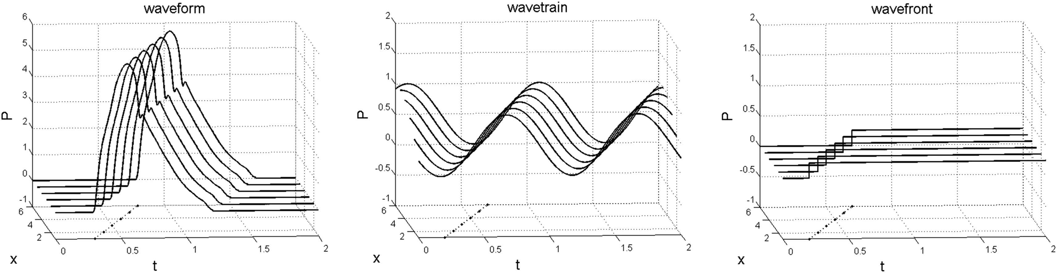
A sketch of the different ‘waves’ as defined in this paper. (left) ‘Waveform’, (middle) ‘wavetrain’, (right) ‘wavefront’. Pressure and time are in the plane of the paper so that each curve represents the pressure waveform measured at a particular location. Distance is increasing into the page so that all of the waves are travelling in the positive direction. The wavefronts shown to the right of this figure are the elemental waves in the following discussion. The dots in the x–t plane indicate the ‘feet’ of the waves and their slope indicate the wave speed at which they are propagating.
Although the concept of a measured waveform being generated by a series of successive wavefronts may seem unfamiliar, a similar method is used routinely in the generation of lines in digital graphics. As seen in Fig. 2, if we zoom into a digital plot of a pressure waveform, we see that it is actually composed of a series of vertical lines at each pixel in the horizontal direction. If we think of the horizontal pixel as the sampling time and the length of the vertical line as the change in pressure during the sampling time, these are the successive pressure wavefronts that make up the measured pressure waveform. Any waveform can be built up by the appropriate wavefronts including, of course, a sinusoidal wavetrain.
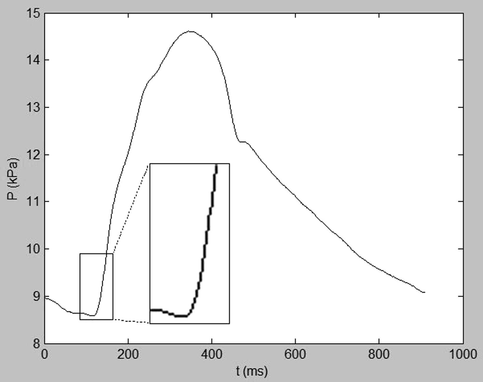
A plot of a pressure waveform in the aorta vs time. Zooming in on the foot of the waveform shows the ‘wavefronts’ as vertical lines for successive intervals of time indicated by the horizontal pixels. If we consider the horizontal pixels as sampling periods, the length of the vertical lines correspond to the magnitudes of the pressure wavefronts.
Four puzzling observations of arterial behaviour
The first observation I would like to consider is what happens when the heart stops beating. Ectopic or missing beats are generally benign and commonly observed in continuous arterial pressure measurements (see Fig. 3, left). In general, the exponentially declining fall in pressure that is commonly observed during diastole simply carries on falling until the next heart beat. In Fig. 3 (right), we see that this exponential fall continues even when the heart is stopped for extended periods, in this example by external fibrillation.20 I believe that this behaviour is crucial for the understanding of arterial hemodynamics and, because it is transient in nature, it cannot be studied using Fourier analysis.
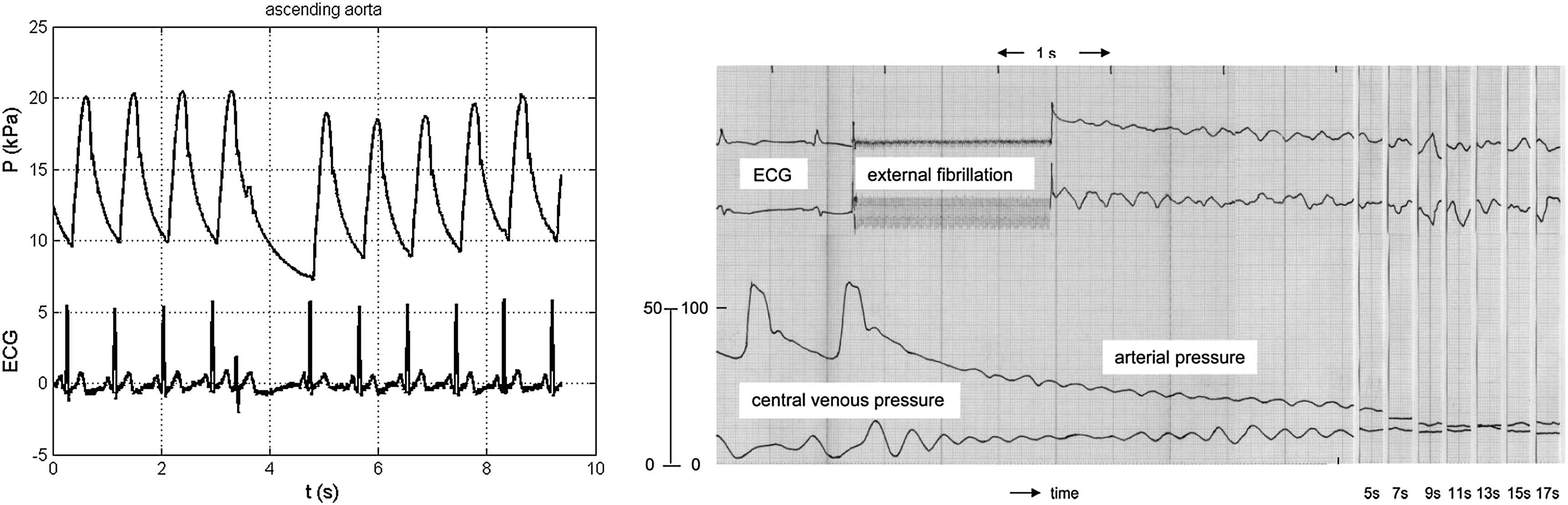
(Left) Pressure measured in the ascending aorta during a missing beat at approximately 4 s. Note that the exponentially falling pressure during diastole in the preceding beat carries on falling during the missing beat. (Right) Pressure measured in the aorta of a patient during two normal beats and an extended period after the cessation of the heart beat due to the application of external fibrillation. Note that the pressure continues falling more or less exponentially during the whole of the 17 s before the heart was defibrillated.20
The second observation comes from a study performed by Westerhof and his colleagues more than 40 years ago.32,33,26 They measured the effect of a total occlusion of an artery on the pressure P and volume flow rate Q measured in the ascending aorta. The four occlusion sites in the aorta were at the aorto-iliac bifurcation (low), at the level of the renal arteries (mid), at the level of the diaphragm (dia) and where the aorta leaves the vertebral column (high). Their results (Fig. 4) show large changes in the ascending aorta in P and Q and the input impedance
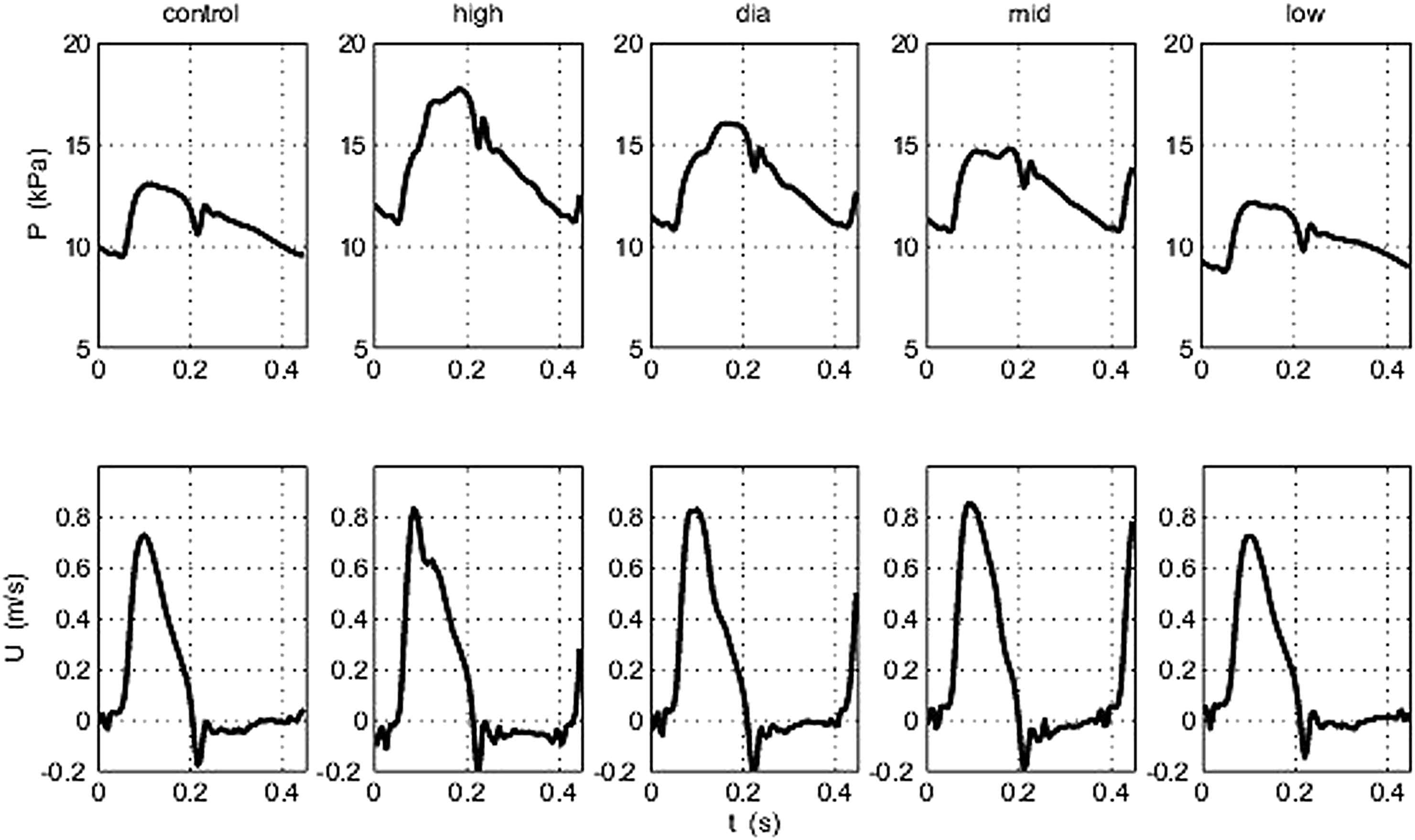
Pressure and velocity measured in the ascending aorta of a dog during total occlusion of the aorta at different locations: (control) no occlusion, (high) upper descending aorta, (dia) at the level of the diaphragm, (mid) at the level of the renal arteries and (low) at the aorto-iliac bifurcation.26
The third observation comes from an even older theoretical study by M.G. Taylor who calculated the input impedance of a number of randomly generated arterial networks.24 Each of the networks was a symmetrically branching tree composed of 7 generations with 128 final branches terminating in identical resistances. The random element of the study comes from the choice of the lengths of the vessels which, in each generation, were drawn from a gamma distribution. The mean length of each generation as well as their cross-sectional area and wave speed were chosen to ‘represent a reasonable model of a generalized arterial system’. As seen in Fig. 5, the calculated impedance spectra of the different networks are very different, except for the values at the fundamental and the first few harmonics which are remarkably similar. Taylor observed ‘…the main and important feature of a steep descent from the value of the terminal impedance at ω = 0, is common to all three realizations of the branching assembly.
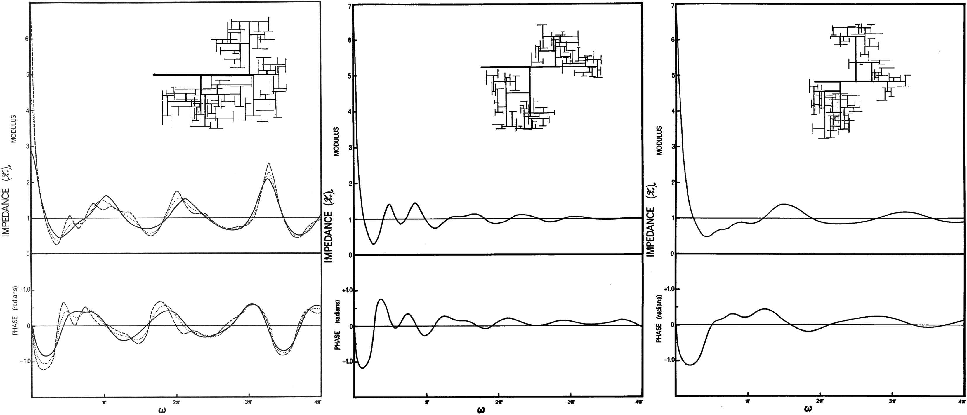
The input impedance of three different assemblies of randomly branching elastic tubes. The cross-sectional area, wave speed and mean length of all vessels in each generation are identical and vary from generation to generation in a physiologically reasonable way. The lengths of the vessels in each generation are drawn randomly from a gamma distribution. The different networks are shown in the upper right of each plot. The curves are the magnitude and the phase of the input impedance power spectrum. The dotted and dashed curves in the figure to the left show the effect of changing the terminal resistances. These results and other calculations in which the fluid and wall viscosity were varied indicate that the geometry of the network is the main determinant of the input impedance.
The final observation comes from recent measurements in dogs by Wang et al.30 They made sequential measurements of P and Q at regular intervals along the aorta, starting in the ascending aorta. Measurements like these have been made by many researchers over the years. The novel aspect of this study is that they separated the measured pressures into forward and backward waveforms. In their study they used wave intensity analysis for the separation but identical results would result from an impedance analysis of the data.11 We have repeated similar measurements in humans with identical results. As seen in Fig. 6 (left), the pressure waveforms measured every 10 cm down the aorta, starting approximately 5 cm from the aortic valve, vary in shape and pulse pressure. These waveforms are similar to other measurements in man and in animal models and the time of the maximum dP/dt at each location in the x–t plane clearly shows that they are propagating down the aorta. The right figure shows the pressure waveforms separated into their forward (blue) and backward (red) components. During early systole the forward wave is virtually identical to the measured pressure and it is clearly propagating down the aorta. The backward pressure wave begins to rise after a short delay in a way that is consistent with the backward wave being a reflection of the initial forward wave from distal locations. However, noting the time of the maximum dP/dt at each location, it is clear that it is also propagating forward with dP/dtmax occurring later at the more distal measuring sites. This result of a forward-travelling backward wave is a serious contradiction. This and other anomalies led us to a reconsideration of the reservoir nature of the arterial system, the main topic of this paper. First, however, it is necessary to review some previous work on wave intensity analysis.
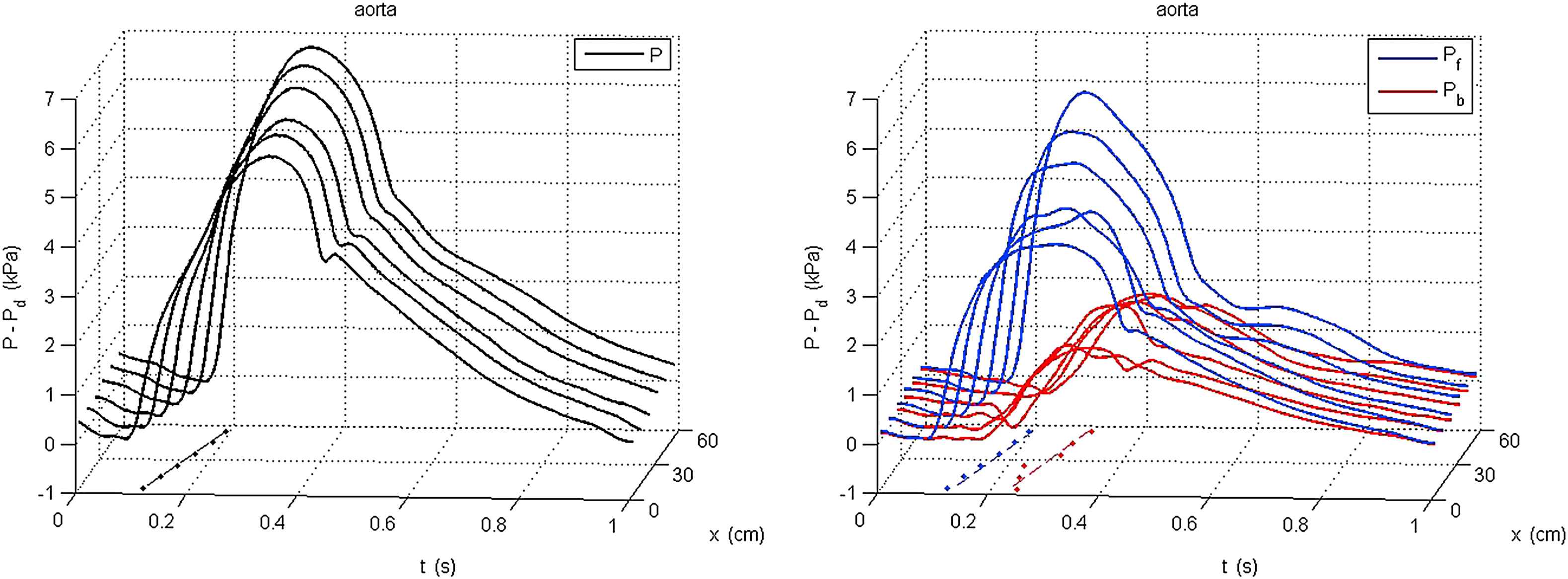
Plots of the pressure measured every 10 cm down the aorta. For ease of comparison P − Pd is plotted where Pd is the diastolic (minimum) pressure at each site. (Left) the measured P − Pd (black). (Right) measured P − Pd (grey), the forward component Pf − Pd (blue) and the backward component Pb − Pd (red). In both figures the dots in the x–t plane indicate the time of dP/dtmax of the individual curves and the dotted line is a linear line fitted to them. The slope of the dotted line corresponds to the wave speed.
Wave intensity analysis
Wave intensity analysis (see17 for a fuller introduction) is based on the 1-D conservation equations for flow in a flexible tube. If the tube has uniform properties along its length, the conservation of mass and momentum require
Equation (1) is the conservation of mass in a differential element of the tube. Physically it says that the rate of change of the volume of the element is equal to the difference between the volume flow Q = UA into the element and the volume flow out of it. It is based on the reasonable assumption that blood is incompressible. Equation (2) is the conservation of momentum for the blood flowing through the element. Physically it says that the net acceleration of the blood, the left hand side, is equal to the combined pressure and wall shear stress forces per unit mass, Newton’s second law. These two equations involve three dependent variables P, U and A and so another relationship is necessary to enable solution. This is provided by a ‘tube law’ which relates A and P through the material properties of the wall.
The resulting equations are hyperbolic in form which means that they can be solved using the method of characteristics due to Riemann. The mathematics involved are rather complex but the practical results of solution are rather simple and very useful. Briefly, the theory tells us that:
- 1)
Any change imposed on the vessel will generate wavefronts that will propagate at speeds U ± c, where c is the wave speed. The theory also shows that c = 1/ρD where
- 2)
There is a relationship between the pressure change dP caused by the wave and the velocity change dU. This relationship is given by the ‘water hammer’ equations dP± = ± ρcdU±, where ‘+’ refers to the forward and ‘−’ the backward travelling waves. A wavefront can be either compressive (dP > 0) or decompressive (dP < 0), accelerating (dU > 0) or decelerating (dU < 0). From the water hammer equations we see that forward compression waves accelerate the flow and forward decompression wave decelerate the flow. Similarly backward compression waves decelerate the flow and backward decompression waves accelerate the flow.
- 3)
It is possible to determine the direction of a wave from the magnitude of its wave intensity dI = dPdU; all forward waves have dI > 0 and all backward waves have dI < 0. It can also be shown that the net wave intensity is equal to the sum of the wave intensities of the forward and backward waves that intersect at that particular time and place in the vessel, dI = dI++dI−.
- 4)
If the waves are additive, which can almost always be ensured by taking sufficiently small sampling times, the water hammer equations can be used to find the forward and backward pressure waves from the simultaneously measured pressure and velocity, dP± = (dP ± ρcdU)/2. From the pressure waves, the water hammer equations can be used to find the velocity waves, dU± = ±dP±/ρc.
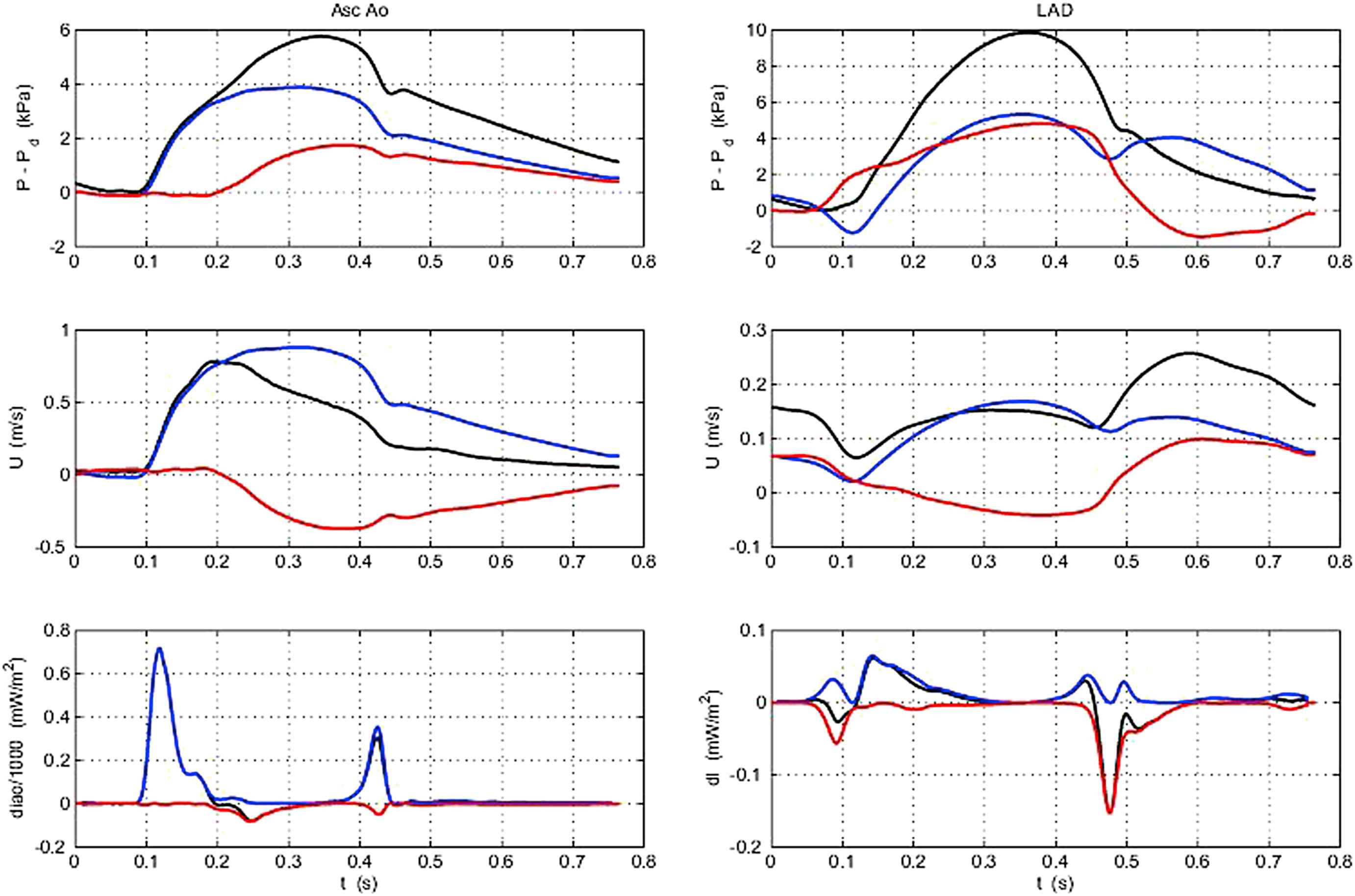
Figure 7 illustrates the utility of wave intensity for interpreting the magnitude and direction of waves in the arteries from simultaneous measurement of P and U. In the ascending aorta (left) we see that there are two positive peaks in the wave intensity indicating periods when forward waves are dominant. The first peak is a forward compression wave (increasing P and increasing U) corresponding to the initial ejection wave at the start of systole. The second, smaller positive peak is a forward decompression wave (decreasing P and decreasing U) that is generated by the left ventricle as it begins to relax at the end of systole. There is a small negative peak in mid-systole which corresponds to a time when P is increasing but U is decreasing. This is due to the effect of backward waves generated by the reflection of the forward compression wave from various sites in the arterial system. The lack of larger reflected waves in the ascending aorta was initially unexpected. Measurements in more distal arteries tend to show larger negative peaks corresponding to larger backward waves in mid-systole.36
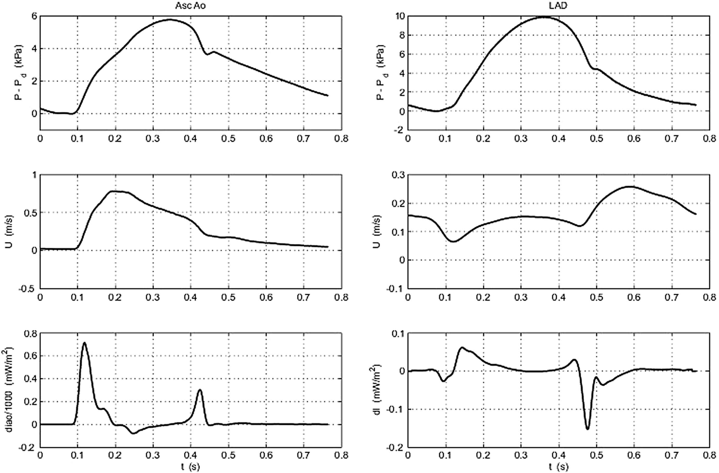
Plots of the measured pressure (top) and velocity (middle) and the calculated wave intensity (bottom) measured in the ascending aorta (left) and in the left anterior descending coronary artery (right).
It should be remembered that decompression wavefronts will also reflect and so we should expect similar reflected waves from the forward decompression wave generated at the end of systole. Because this wave is generally smaller than the initial compression wave associated with the start of ejection, these backward waves are generally not very prominent, but their existence should be recognised.
In the coronary arteries (right) the pattern of wave intensity is much more complex. The contraction of the myocardium at the start of systole has two effects. Contraction during the isovolumetric contraction period will cause a small backward wave (just visible) due to the compression of the intramural coronary arteries which precedes ejection. Compression of the intramural arteries will continue during ejection generating backward compression waves which will, to some extent, be overcome by the forward compression waves propagating into the coronary artery from the aorta that are associated with ejection. In the measurements shown in Fig. 7 (right), the first peak after the start of systole is negative indicating that the backward waves generated by compression of the distal vessels arrive at the measuring site before the forward waves transmitted through the aorta arrive forming the second, positive peak in dI. The largest peak is the negative peak at the end of systole which indicates the arrival of backward decompression waves that are ‘sucking’ blood into the coronary vessels as the myocardium relaxes. This is the source of the large acceleration seen at the start of diastole causing the coronary perfusion to be mostly out of phase with the coronary artery pressure. Being able to relate the strength and direction of arterial waves to the temporal changes in the myocardium during the cardiac cycle is one of the benefits of wave intensity analysis.
Instantaneous wave-Free Ratio (iFR)
This ability of wave intensity analysis to reveal the timing and magnitude of waves in the arteries has recently been exploited to assess the functional severity of coronary stenosis.21,22 Under steady flow conditions, the resistance to flow of the stenosis can be determined by measuring the pressure drop across the stenosis or, equivalently, the ratio of the downstream and upstream pressures. In the highly dynamic coronary arteries this ratio is highly variable and depends in a complex way on the variation of the microcirculatory resistance as the myocardium contracts and relaxes. Currently the standard clinical measure of the hemodynamic severity of a coronary stenosis is the Functional Flow Reserve (FFR) defined as the ratio of downstream and upstream pressures during maximal hyperemia induced by the injection of a vasodilator, usually adenosine. From wave intensity analysis, we see that there is generally a period during diastole which is wave-free when the microcirculatory resistance in minimal and effectively constant and consistent from beat to beat (Fig. 8, left).
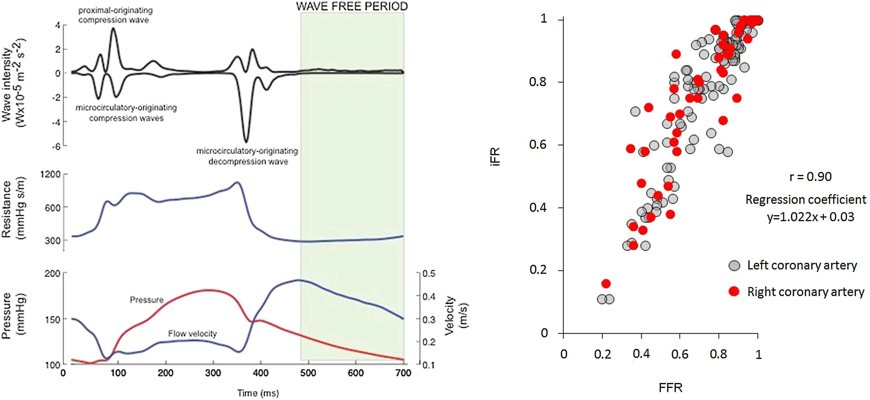
(Left) The bottom trace shows P (red) and U (blue) during one cardiac cycle measured in a stenosed coronary artery, showing that coronary flow is smallest during systole and maximal during diastole. The middle trace shows the resistance calculated as the ratio P/U, showing how the microcirculatory resistance varies during systole. The top trace shows the wave intensity calculated from the simultaneously measured P and U separated into its forward (positive) and backward (negative) components. The wave-free period (shaded) occurs during diastole when the resistance is minimal and effectively constant. (For interpretation of the references to colour in this figure legend, the reader is referred to the web version of this article.)
The instantaneous wave-Free Ratio (iFR) is defined as the ratio of downstream and upstream pressure during this wave-free period. This ratio compares very well with the FFR measured after the administration of adenosine (Fig. 8, right). The advantages of iFR for the clinical measurement of coronary artery stenosis are obvious: adenosine has unpleasant side-effects, is expensive and prolongs the duration of the investigation significantly. Most importantly, iFR can be measured repeatedly during the catheter session allowing for assessments before and after stenting or the sequential assessment of multiple stenoses.
Separation into forward and backward waves
The separation of P and U waves into their forward and backward components is an old32 and generally accepted approach to arterial hemodynamics.11 Fig. 9 shows the P, U and dI data in Fig. 8 separated into their forward and backward components. The separated wave intensity does not add much information to that obtained from the net wave intensity in the ascending aorta because the peaks are widely separated so that the net and separated curves tend to coincide. This is not true in the coronary arteries where we see there are periods, particularly at the start of systole, where there are relatively large simultaneous forward and backward waves which cancel each other giving relative small net wave intensity.
Plots of the pressure, velocity and the wave intensity (shown in Fig. 8) measured in the ascending aorta (left) and in the left anterior descending coronary artery (right); (black) measured data, (blue) forward components, (red) backward components. (For interpretation of the references to colour in this figure legend, the reader is referred to the web version of this article.)
The Windkessel model
The storage of blood in the compliant arteries during systole and its release during diastole was first described by Borelli in the 17th century4 and more fully by Hales in the 18th century,9 who compared it to the air chamber used in fire engine pumps of his day to help smooth the outflow of water from the hose. The idea was made quantitative by Frank at the very end of the 19th century,7 who translated Hales’ analogy into ‘Windkessel’ and this is the name that is generally used to describe the phenomenon. The Windkessel pressure as defined by Frank is derived from a simple two-compartment model of the arterial system. Mass conservation of the incompressible blood requires that the rate of change of the volume of the arteries dV/dt is equal to the difference between the volume rate of flow out of the heart into the arteries Qin and the volume flow out of the arteries through the microcirculation Qout.
This equation is identical in principle to Eq. (1). Both equations express the conservation of mass in different control volumes; the entire arterial system in Eq. (3) and a differential element of a single artery in Eq. (2).
Assuming that the net compliance of the arteries is constant C = dV/dP and that the flow through the microcirculation is resistive in nature
This equation can be solved by quadrature for any Qin(t). In particular, we see that during diastole when Qin = 0 the solution is
The simple Windkessel theory suffers from a fundamental physical problem. The assumption that there is a uniform pressure throughout the arterial system that comprises the Windkessel is not possible because of the wave nature of the arteries; it takes time for the conditions imposed by the ventricle at the aortic root to propagate through the arterial system. The only way to have a uniform pressure would be for the wave speed to be infinite. However, because the wave speed is inversely related to the distensibility of the artery, an infinite wave speed implies zero distensibility. This means that the Windkessel model is valid only if there is no Windkessel effect.
Reservoir and excess pressure
We introduced the reservoir-wave hypothesis over a decade ago27 defining the ‘Windkessel’ and ‘wave’ pressures. As our ideas matured we renamed them as the ‘reservoir’ pressure, to acknowledge that our concept of the reservoir pressure is subtly different from Frank’s definition of the Windkessel pressure, and the ‘excess’ pressure, to avoid the impression that the excess pressure was solely responsible for arterial waves. The basic concept of the reservoir-wave hypothesis has been discussed in a number of more recent papers.5,25 Although there is currently no universal agreement about the proper definition of reservoir pressure Pr, I will define it as a time-dependent pressure that is uniform throughout the large arteries but is delayed at any particular location by the wave travel time from the aortic root to that location. The excess pressure Pe at any location is simply the difference between the reservoir pressure and the measured pressure.
Importantly, we require that Pr be a solution of the net conservation of mass for the arterial system,
Historically there are different definitions of the reservoir pressure.b The first definition is simply the local Windkessel pressure calculated from the locally measured flow rate Q, which is assumed to correspond to Qin, as the solution to the 1st order ODE.27
In order to apply the reservoir wave hypothesis to clinical measurements, we proposed an algorithm for calculating the reservoir pressure using only the locally measured pressure.1 This algorithm is based on two assumptions; Pr(t) is uniform throughout the arterial system and the observation in the ascending aorta of dogs that the calculated excess pressure is virtually identical in form to the measured flow rate.27 If we assume that Pe = σQ0, then the reservoir pressure can be calculated as the solution to the 1st order ODE
The value of σ is obtained either by matching the solutions during systole and diastole at the time of the end of systole or, more recently, by finding the value of σ that maximises the fit over the whole of the cardiac period. Over the years we have refined this algorithm so that it is very robust and completely objective. Although we have not yet published the details of this algorithm, it is available as a Matlab code upon application to the author. It is this algorithm that has been used to calculate the reservoir pressures in the examples in this paper.
In a recent work, we needed a mathematically precise definition of the reservoir pressure rather than an algorithmic definition.18 We considered the pressure in a network of arteries with a given flow into the aortic root Q0(t). We made the basic assumption that the reservoir pressure is identical throughout arterial network but delayed by the time taken for a wave to travel from the aortic root to a particular vessel τn. Further assuming that the compliance of each vessel in the network Cn and the resistance at the end of each terminal vessel Rn are known, we used the global continuity equation to define Pr
The lack of a well-agreed definition of the reservoir pressure is a drawback, but it does not negate the possibility that it is a useful concept for the analysis of arterial mechanics. Given the complexity of the arterial system and the global nature of Pr, a formal definition will almost certainly depend upon a level of knowledge about the local arterial properties throughout the network that is impossible to realise clinically. This is similar to the problems faced by the application of numerical models of arterial hemodynamics where, for example, a relatively simple 1-D model based on the 55 largest arteries requires knowledge of approximately 300 properties such as the length, diameter, taper, elastic modulus, etc. of each vessel.3,19 The goal of much of our current work is to find an approximate, clinically useful definition of the reservoir pressure Pr and, thereby, the excess pressure Pe.
Resolving the puzzles – the usefulness of the reservoir pressure
The existence of reservoir pressure raises thorny philosophical questions. Most mathematicians would argue that reservoir pressure exists simply because it has been defined. Other, more practical people would prefer a more physical verification. In any case we can question the usefulness of reservoir pressure as a concept. Here we will discuss some of the benefits of dividing the measured arterial pressure into a reservoir and an excess pressure. Some of the benefits are immediately obvious, others are more speculative but still worth exploring.
The usefulness of the reservoir pressure is obvious when we consider the behaviour of the arterial pressure when the heart stops beating. Figure 10 shows the pressure measured in the aorta (solid lines) together with a projection of the pressure of each beat assuming that the next beat did not occur (dashed lines). Looking at the emphasised beat at about 5 s, we see that more than half of the diastolic pressure at the end of the beat is contributed by the previous beat and that earlier beats contribute to this pressure in an exponentially falling way. Since the reservoir pressure provides a very good approximation to this behaviour, it follows that the excess pressure is representative of the hemodynamics within the beat, independent of previous beats. Therefore, the reservoir pressure will be primarily dependent upon heart rate and the global arterial properties while the excess pressure will depend on local conditions and variations in ventricular contraction.
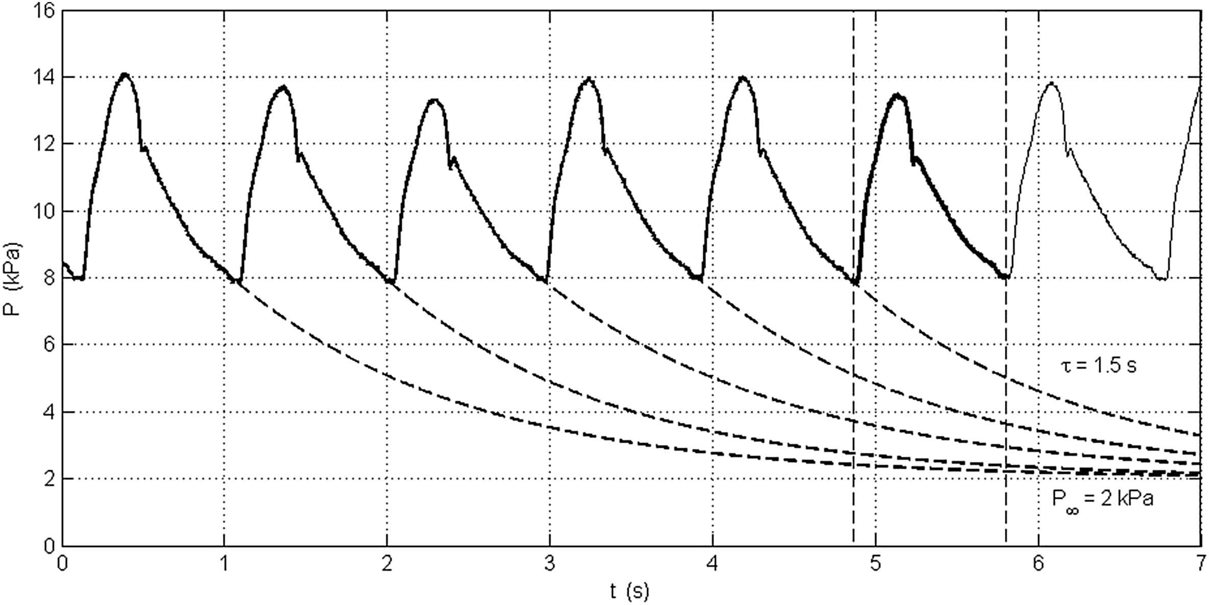
Pressure measured in the aorta over 7 s (solid line). The pressure during diastole of each beat has been fitted by an exponentially falling pressure of the form P(t) − P∞ = (P0 − P∞)e−t/τ, where τ is the time constant and P∞ is the asymptotic pressure (assumed to be 2 kPa). The dashed line indicates the pressure that would be observed if the succeeding heart beats did not occur. We see for the sixth (emphasised) beat that a significant fraction of the diastolic pressure is contributed by previous beats.
The observation by Westerhof and his colleagues that occlusion of the distal aorta resulted in immeasurably small changes at the ascending aorta is not directly explained by the reservoir/excess pressure hypothesis but follows from related observations about the nature of arterial bifurcations. The reflection coefficient Γ at a bifurcation depends upon the characteristic impedances Za, Zb and Zc of the three vessels comprising the bifurcation
It has been observed by many that the anatomical and mechanical properties of the large arteries are such that they are approximately ‘well-matched’ for forward travelling waves.15 That is to say Γa ≈ 0 when a is the parent vessel. It follows, however, that a bifurcation which is well-matched in the forward direction cannot be well-matched in the backward direction which means that much of the energy of a wave approaching a bifurcation in one of the daughter vessels will not propagate into the parent vessel. For example, a symmetrical bifurcation that is well-matched in the forward direction Γa = 0 will have a reflection coefficient Γb = −0.5 for a backward travelling wave in vessel b. The effect of this asymmetric propagation of waves in the human aorta is shown in Fig. 11. The figure shows the transmission coefficients for forward waves (left) and backward waves (right) calculated for the major bifurcations in the aorta using data published in Refs. 31,23 The net gain for forward waves, 1.07, indicates that the aorta is very close to well-matched in the forward direction. The net gain for backward waves, 0.15, indicates how poorly backward waves are transmitted as the travel up the aorta. This, I believe, is the explanation for the observations of Westerhof et al. in their 1970 experiment (Fig. 4).
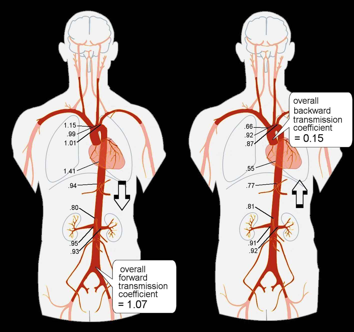
The forward (left) and backward (right) transmission coefficients at the major aortic bifurcations between the heart and the iliac bifurcation. The coefficients are calculated using data collected in Refs. 31,23 The net gain is the product of all of the transmission coefficients. The net gain for forward waves, 1.07, indicates that they travel from the heart to the iliac bifurcation with minimal change. The net gain for backward waves, 0.15, indicates that they are strongly diminished by reflections as they travel from the distal end of the aorta to the heart.
Taylor’s theoretical observations of the input impedance for randomly generated arterial trees also provides support for the idea of a reservoir pressure. Because of the way that he constructed his models, the total peripheral resistances of each of his random networks is constant but the net compliance, depending on the randomly selected lengths of the vessels in each generation, will vary from network to network. An essential part of the definition of reservoir pressure is that it satisfies the global conservation of blood volume. Taking the Fourier transform of the ODE describing mass conservation results shows that the input impedance due to the reservoir effect will have the form
The usefulness of the reservoir/excess pressure in resolving the anomaly of forward travelling backward waves in the aorta is obvious in Fig. 12 which shows the data seen in Fig. 6 separated into reservoir and excess pressure (left) and the excess pressure further separated into its forward and backward components (right). Several features of these data should be noted. Pr (green) calculated from the pressure waveforms P at each measurement site are remarkably similar in shape but delayed by the wave travel time from the inlet of the aorta to the measurement site. During systole there is a large variation in the excess pressure Pe at the different measurement sites reflecting the change in the pressure waveform as it propagates down the aorta. During diastole Pr is virtually identical to P which means that the excess pressure Pe is nearly zero throughout diastole. Finally, we see in the figure on the right that the forward component of Pe is very similar to Pe while the backward component is very small. This is consistent with our observations about the well-matched nature of the aorta for forward travelling waves and the poor transmission of backward waves seen in the occlusion experiments of Westerhof et al.
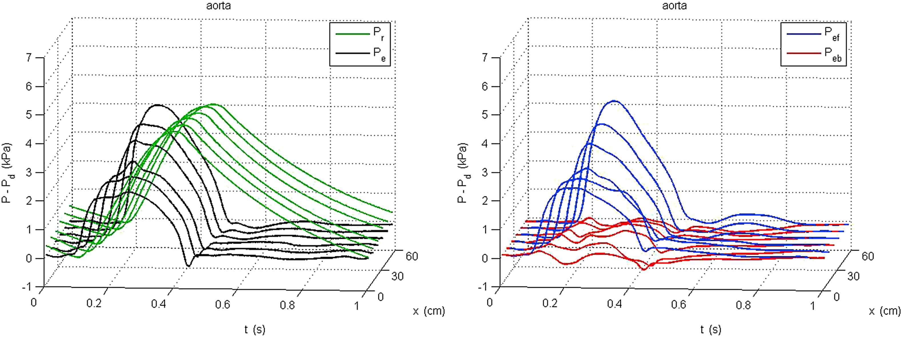
Plots of the reservoir and excess pressure calculated from the pressure measured every 10 cm down the aorta shown in Fig. 6. The figure on the left shows the reservoir pressure Pr − Pd (green) and excess pressure Pe − Pd (black). In the figure on the right, the excess pressure is separated into its forward component Pef − Pd (blue) and backward component Peb − Pd (red). The backward component is noisy because of the noise inherent in the measurement of the aortic velocity, but the distinct forward travelling nature of the backward wave seen in Fig. 6 is no longer present. (For interpretation of the references to colour in this figure legend, the reader is referred to the web version of this article.)
Discussion and conclusions
In addition to its usefulness in explaining various observations about arterial behaviour discussed in the previous section, the reservoir/excess pressure has shown some clinical promise in preliminary studies. Wang et al.29,30 showed that vasodilatation by nitrates and vasoconstriction by methoxamine had different and complex effects on the aortic reservoir pressure. The fraction of left ventricular work attributed to the reservoir pressure was strikingly different before and after the administration of the drugs.
Although all of the discussion in this paper has been about the arterial reservoir pressure, it is also possible to extend the concept to the venous system. In the systemic veins, the input flow is the flow from the arteries through the microcirculation and the outflow is the flow into the right atrium which results in an exponentially growing venous pressure during diastole. We have applied the reservoir-excess pressure separation to measurements made in dogs with very promising results.28 Just as we found that the excess pressure waveform in the ascending aorta was virtually identical to the flow from the left ventricle, the excess pressure waveforms in both the superior and inferior vena cava were virtually identical to the measured flow out of these central veins. This result is very interesting because it suggests a new approach to the study of venous hemodynamics, a sorely neglected area of study.
One of the more exciting results comes from an as yet unpublished analysis of the reservoir and excess pressures calculated from the radial artery pressure tonometry measurements made in the Conduit Artery Functional Endpoint (CAFE) study, a prospective study of cardiac events in hypertensive patients on atenolol- or amlodipine-based therapy which was a substudy of the Anglo Scandinavian Cardiac Outcomes Study (ASCOT).6 In the study 2069 hypertensive patients were allocated randomly to the two treatment arms and the dosage was adjusted until their brachial blood pressure achieved target values. They were followed over a median of 3.4 years. In this group, the integral of the excess pressure over a cardiac period (XSPI) was a significant predictor of cardiovascular events. It remained a significant predictor after adjustment for other, conventional risk factors such as age, sex or Framingham risk score.
More recently we have calculated the reservoir/excess pressure from central pressure measurements derived from radial pressure tonometry measurements in a cohort of 674 high-risk patients with preserved left ventricular function.10 The patients were followed for a median of 1395 days. In these patients both the backward wave calculated from the measured pressure and the reservoir pressure were significant predictors of cardiac events. A subsequent analysis showed that there was an extremely high correlation between the backward pressure wave and the reservoir pressure which is to be expected because the reservoir pressure is highly dependent on the measured pressure during diastole and the backward pressure must equal half of the measured pressure to ensure zero flow during diastole.
A theoretical study showing that the reservoir pressure is the waveform that results in the minimum left ventricular hydraulic work for a given flow waveform18 is a good indication of the potential usefulness of reservoir and excess pressure clinically. Achieving the reservoir pressure waveform physiologically would require an extraordinary matching of vessel impedances and terminal resistances that is probably not possible because of other constraints on the cardiovascular system. However, even if the reservoir pressure cannot be realised physiologically, this result suggests that it can be useful reference for the assessment of cardiac efficiency. The analysis of the efficiency of man-made pumps and engines frequently relies upon unrealisable, ideal performance cycles (the Carnot cycle for steam engines, the Otto cycle for internal combustion engines, the Brayton cycle for jet engines, etc). If the reservoir pressure results in the minimum possible hydraulic work for a given flow from the heart and given properties of the arterial system, then the work done against the excess pressure is excess work over and above the ideal minimum. It seems reasonable that minimising the excess work done by the failing heart will be therapeutic, which is consistent with the CAFE study results.
The lack of an agreed definition of reservoir pressure is inconvenient with each of the definitions having its advantages and disadvantages: The definition introduced by Wang et al. (Eq. (8)) is a straightforward local application of Frank’s Windkessel analysis which requires clinically unfeasible simultaneous measurements of local pressure and velocity; the algorithmic definition of Aguado et al. (Eq. (9)) allows the calculation of the reservoir pressure from the measured pressure alone, but is based on a number of assumptions that need to be tested further; and the mathematical definition used by Parker et al. (Eq. (10)) is precise but requires god-like knowledge of the mechanical properties of the entire arterial network that makes it impossible to measure clinically. It is possible that these definitions may continue to be useful in different circumstances – an ‘effective’ reservoir pressure that can be measured clinically and a ‘mathematical’ reservoir pressure that can be used in theoretical models. In any case, it is crucial that the definition of the reservoir pressure requires it to obey the condition of overall conservation of mass in the arterial system.
It can be argued that there is an analogy between the reservoir pressure in the hemodynamics of the arteries and the motion of the centre of mass in the mechanics of the body (see the Appendix: Jumping analogy). Using Newton’s Third law, it is easy to show that the motion of the centre of mass of a body depends only on the net external forces acting on the body and is independent of the relative motion of different parts of the body due to internal forces. Recall that the centre of mass is a theoretical concept which may not even lie within the body (for example, the centre of mass of a horseshoe). No matter how complex the movement of a diver during a dive, the diver’s centre of mass follows the same trajectory it would if the diver was completely passive. Thus, the analysis of body movement is simplest if it is carried out in ‘body coordinates’ moving with the centre of mass. I would argue that the reservoir pressure which obeys the strong condition of overall conservation of mass is analogous to the motion of the centre of mass which obeys the strong condition of overall conservation of momentum.
In conclusion, I would refute critics of the reservoir-excess pressure hypothesis who say ‘the reservoir pressure does not exist’ by saying that its existence depends upon its usefulness as a concept. We have shown how the concept can resolve anomalies in the current interpretation of a number of observations about arterial behaviour. There are a number of preliminary results that indicate that it provides clinically useful measures in the study of the effects of different drugs and may be a clinical indicator of the risk of cardiovascular events. These preliminary results do not provide conclusive evidence of the utility of reservoir and excess pressures but they do suggest that it is an avenue well worth exploring.
Appendix Jumping analogy
We can make an analogy between the hemodynamics of the arteries and the mechanics of jumping. Consider a person jumping up and down with their arms held horizontally to the side. Assume that we measure the force applied to the ground and the height of the hands as a function of time. If the jumps are periodic we will measure a periodic force and a periodic height and there will be a relationship between them. This relationship will be rather complex because the hands are connected to the shoulder through the bones, ligaments and muscles of the arms, all of which will respond to the applied forces in a complicated way.
The easiest way to analyse this problem is to consider the motion of the centre of mass of the whole body in response to the net force acting on it (the force of gravity and the force applied to the ground by the muscles of the leg during the different phases of the jump; resting, the lift-off phase when the muscles apply a force through the feet to the ground, the ‘free flight’ phase when the feet are off the ground, and the recovery phase when the feet hit the ground again and the leg muscles cushion the shock of landing. From basic theorems of mechanics, we know that the motion of the centre of mass will be determined by the instantaneous forces acting on the whole body, muscle forces and gravity, but will be independent of internal forces acting between different parts of the body. Once we know the motion of the centre of mass, we can consider the motion of the arms in body coordinates moving with the centre of mass. That is, it is convenient to divide the motion of the hands into the motion of the centre of mass plus the motion of the hands relative to the centre of mass.
Figure A1 shows the results calculated for a very simple, idealised example of jumping. It is assumed that the person of mass M jumps regularly 50 times a minute, that a constant force F/M = 3 G’s is generated over a period of 100 ms as the legs contract resulting in a take-off velocity of 2 m/s, that the legs generate an identical force to cushion the landing so that pre-jump crouching stance is reattained 100 ms after touch-down and that the jumper remains motionless until the start of the next jump. The coupling of the arms of mass m to the shoulder is assumed to be a simple spring with a spring constant k chosen so that the natural frequency of the arms,
The height of the hands y in this simple problem is given by the red curve in the lower left panel of the figure. The amplitude of the ratio of the Fourier transforms of F and y (the transfer function) is shown as the red line in the lower right panel. The results are relatively complex even for this very simple example with three significant peaks in the power spectrum. The height of the centre of mass Y is shown in blue in the lower left panel and the transfer function between F and y–Y, the height of the arms in body coordinates, is shown in black in the lower right panel. It is clear that the motion of the hands in body coordinates is very simple with a single peak in the power spectrum at the natural frequency of the arms.
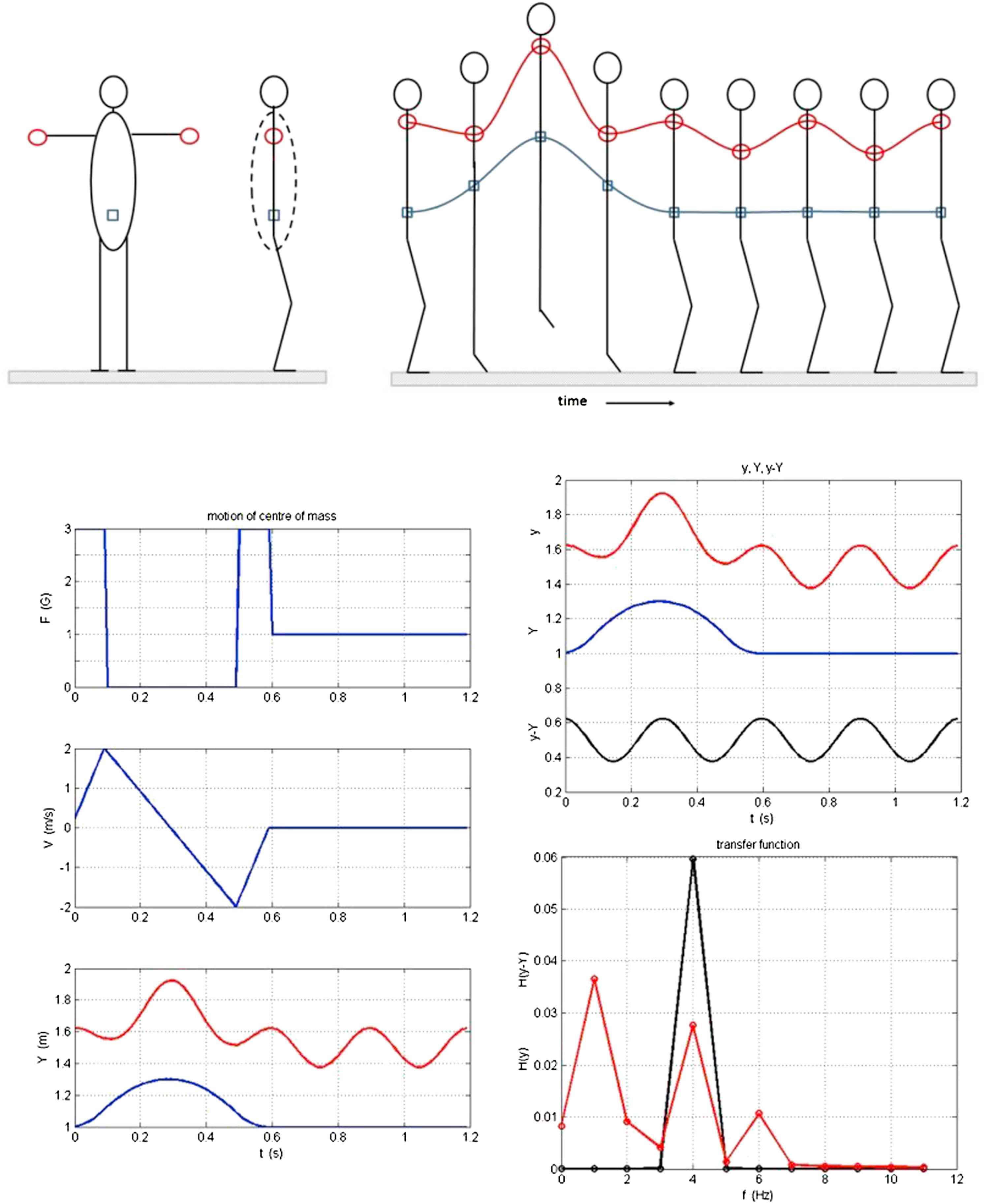
A very simple model of a person jumping 50 times per minute with outstretched arms (top left). The stick figures (top right) indicate different stages of the jump: initiation, leaving the ground, free flight, touch down, absorbing the downward momentum, waiting for the next jump. The position of the hands is given by the red circles and line and the position of the centre of mass is given by the blue squares and lines. The force exerted on the ground (top trace), the velocity of the centre of mass (middle trace) and the vertical position of the hands (red) and centre of mass (blue) are shown in the bottom left figure. The top figure on the bottom right shows the temporal variation of the height of the hands (red), the height of the centre of mass (blue) and the variation of the height of the hands relative to the centre of mass (black). The bottom figure on the bottom right shows the magnitude of the power spectrum of the transfer function between the force applied to the ground and the height of the hands (red) and the transfer function for the height of the hands relative to the centre of mass.
Applying the analogy to the cardiovascular system, the overall conservation of mass in the arteries is equivalent to the overall conservation of momentum for the body as a whole. It is a strong constraint on the system; requiring that the rate of change of the total volume of the arteries is equal to the volume rate of flow into the aorta minus the flow out of the distal arteries through the microcirculation. The reservoir pressure is defined to satisfy this requirement. Therefore, we can argue by analogy that it would be useful to think of the measured pressure as the sum of the reservoir pressure (the motion of the centre of mass) and an excess pressure that accounts for local differences in pressure and flow (the motion of the hands in body coordinates).
Footnotes
In our first paper on the theoretical basis of wave intensity analysis we referred to these waves as ‘wavelets’.16 Unfortunately this word was usurped by mathematicians studying signal processing to mean something entirely different and we have been forced to find a different, and less evocative word.
Another definition of reservoir pressure has been suggested by Alastruey.2 It is based on a 1-D computational model of the arteries and he defines the local reservoir pressure as the pressure due to all of the waves from distal locations. Since he also requires that the total pressure is equal to the sum of the reservoir and excess pressures, this means that the local excess pressure is the pressure due to all of the waves from proximal positions. This definition is interesting theoretically and will certainly contribute to our theoretical understanding of the reservoir pressure. It is, however, difficult to see how it can be applied to experimental measurements.
References
Cite this article
TY  - JOUR
AU  - Kim H. Parker
PY  - 2013
DA  - 2013/10/27
TI  - Arterial reservoir pressure, subservient to the McDonald lecture, Artery 13
JO  - Artery Research
SP  - 171
EP  - 185
VL  - 7
IS  - 3-4
SN  - 1876-4401
UR  - https://doi.org/10.1016/j.artres.2013.10.391
DO  - 10.1016/j.artres.2013.10.391
ID  - Parker2013
ER  -