
The reservoir-wave model☆
This research did not receive any specific grant from funding agencies in the public, commercial, or not-for-profit sectors.
- DOI
- 10.1016/j.artres.2017.04.003How to use a DOI?
- Keywords
- Reservoir pressure; Excess pressure; Low-frequency pressure; Wave front analysis; Eigen-modes; Time constants
- Abstract
This paper is based on a talk given at the Arterial Hemodynamics: Past, Present and Future symposium in June 2016. Like the talk it is divided into three different but related parts. Part 1 describes the calculation of reservoir and excess pressure from clinical pressure waveforms measured at 5 different aortic sites in 40 patients. The main results are that the reservoir pressure waveform propagates down the aorta and is effectively constant from the aortic root to the aortic bifurcation. Part 2 describes a low-frequency asymptotic analysis of the input impedance of an arterial tree. Neglecting terms of second order, the results show that the low-frequency component of the pressure waveform is uniform throughout the arterial tree and is delayed by an effective wave travel time that depends on the properties of the network. The low-frequency pressure waveform shares all of the properties of the reservoir pressure waveform, but it is premature to say that they are identical. Part 3 describes the analysis of arterial hemodynamicsusing wave fronts. It shows that every wave front introduced at the root of the aorta generates an exponentially increasing number of reflected and transmitted waves with exponentially decreasing amplitudes. The long-time response of the arterial tree can be described by a number of exponentially decaying eigen-modes, each with a different time constant. The analysis is applied to a 55-artery model of the human circulation and the modes and their time constants are shown. This theory provides an alternative method for studying arterial hemodynamics and helps in the interpretation of reservoir and excess pressure.
- Copyright
- © 2017 Association for Research into Arterial Structure and Physiology. Published by Elsevier B.V. All rights reserved.
- Open Access
- This is an open access article distributed under the CC BY-NC license.
Introduction
This paper is an outline of the talk given at the meeting Arterial Hemodynamics: Past, Present and Future held at University College London, 14–15 June 2016. It is not a transcript of the talk. It does follow the structure of the talk and is rather more wide ranging than the usual scientific paper, being divided into three slightly disjointed parts. Part 1 describes some recent work analysing clinical arterial pressure measurements taken at five different locations along the aorta using the reservoir-wave model. The full paper describing this work has recently been submitted for publication and so this section takes the form of a brief outline of the main findings. Part 2 describes some recent work analysing the low-frequency component of the pressure wave in an arterial tree using impedance methods. This may seem out of place in a talk dealing with the reservoir pressure hypothesis, but I hope that its relevance is clear in the end. Part 3 concerns current work looking at arterial hemodynamics using wave fronts as the basis of the analysis. Some of the analysis presented at the meeting has now been revised and this outline is based on the most recent results. This analysis shows potential but is not completed and so this part of the paper should be considered to be work in progress rather than final results.
Reservoir and excess pressure along the human aorta
The definition and separation of pressure
Pressure is a such a familiar concept that we frequently forget how it is defined scientifically. In thermodynamics pressure P is defined as
In mechanics the formal definition of P is
Pressure is frequently divided into component parts. Probably the most common division of pressure is the gauge pressure
It is possible to define an absolute pressure Pabsolute. However, this is frequently inconvenient because we usually function in a sea of atmospheric pressure. For this reason we generally use pressure to mean the pressure relative to some reference pressure, i.e. a gauge pressure. This is common practice in the catheter lab where the pressure transducer is calibrated to some pressure relative to the heart which includes the atmospheric pressure. I do not know of any clinic that routinely records the atmospheric pressure which means that it is practically impossible to explore the effect of absolute pressure in hemodynamics.
The most famous separation of pressures into different components is undoubtedly the Bernoulli equation
In the context of this meeting, undoubtedly the most common separation of pressure into different components is the separation of the arterial pressure waveform into its forward and backward components shown in Fig. 1. This follows from the work by Westerhof and his colleagues who showed that simultaneous measurements of the pressure and flow waveform could be used for the separation through calculation of the reflection coefficient.1 A few years later Laximinarayan, working in Westerhof’s group, showed that the separation could be made more conveniently using the characteristic impedance.2 I suspect that everyone attending this meeting has made use of this result in their work. In the separation, it is unclear how to apportion the zeroth component (the steady pressure and flow) between the forward and backward waveforms. Westerhof et al. cleverly got around this problem by letting the forward and backward waveforms drift relative to the scales of their measured counterparts. Laximinarayan resolved the problem by not showing any scales at all. This observation, seemingly trivial, is actually important and has a bearing on the definition of the reservoir pressure.
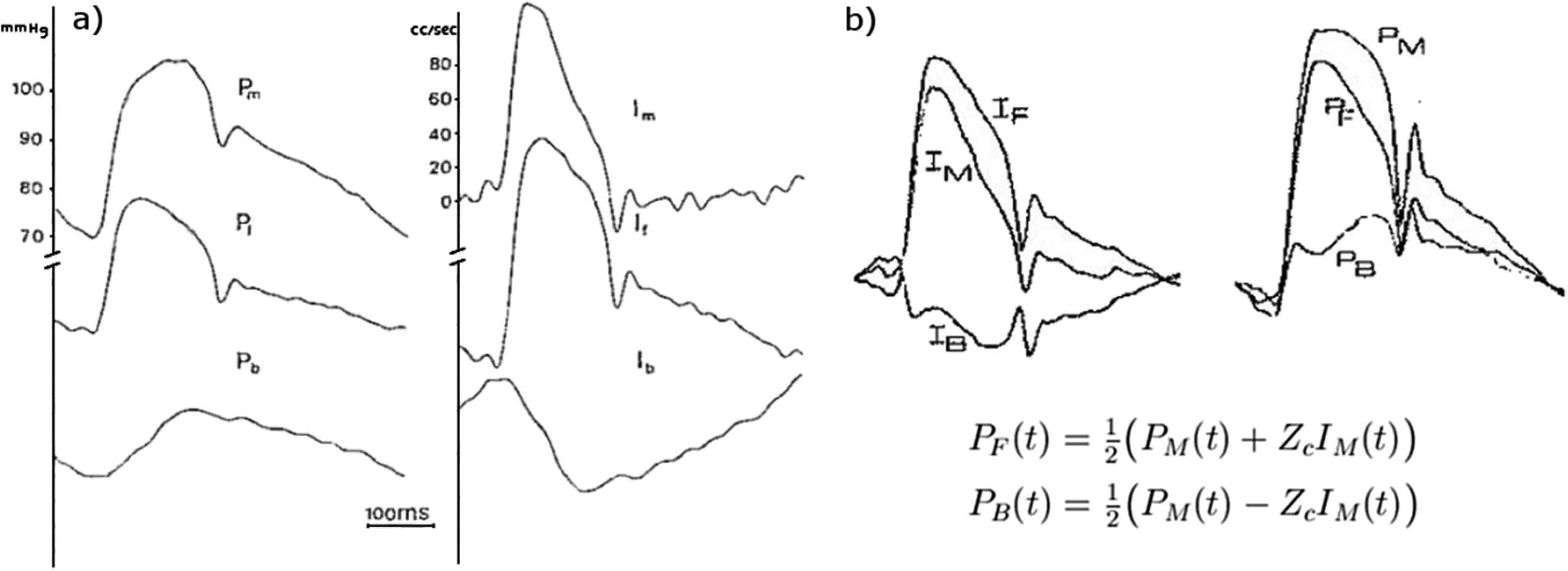
More than a decade ago, we formulated the reservoir-wave hypothesis that it might be useful to divide the measured arterial pressure into a reservoir pressure and an excess pressure defined as the difference between the measured pressure and the reservoir pressure.3 Our argument was based on the success of the Windkessel model in describing the diastolic pressure waveform and in the original paper we separated the pressure into a ‘Windkessel’ pressure and a ‘wave’ pressure. After publishing that paper we realised that the Windkessel pressure was, by definition, uniform throughout the arterial system and could not describe the observed propagation of this component of the pressure down the aorta. For this reason in subsequent papers we defined the ‘reservoir’ Pr and ‘excess’ Px pressures.4
One of the unexpected observations of our experimental work was that the excess pressure waveform derived by subtracting the reservoir pressure from the measured pressure was very similar in shape to the flow waveform at the aortic root. Assuming that this similarity is always true, it is possible to derive the reservoir pressure from the measured pressure alone.a
This ‘pressure-only’ algorithm has been used to retrospectively calculate the reservoir and excess pressure waveforms from measured arterial pressure waveforms in a number of clinical studies which have shown that various parameters related to these pressures are significant risk factors for various cardiovascular events.7–9 These studies indicate that reservoir pressure is, indeed, a useful concept, but that is not the topic of this talk.
Reservoir and excess pressure in the human aorta
One of the primary assumptions in the definition of reservoir pressure is that it is uniform throughout the arterial system and is determined by the global compliance and resistance. The excess pressure, on the other hand, varies at different locations in the arteries and is dominated by local waves. The uniformity of the reservoir pressure is observed in the measurements of pressure and flow at different locations in the dog. It has not, however, been tested in man. Recently we had the opportunity to analyse high fidelity pressure measurements made at 5 different arterial locations in 40 patients. This work has recently been written up and submitted and I will only discuss a few of the relevant results here.10
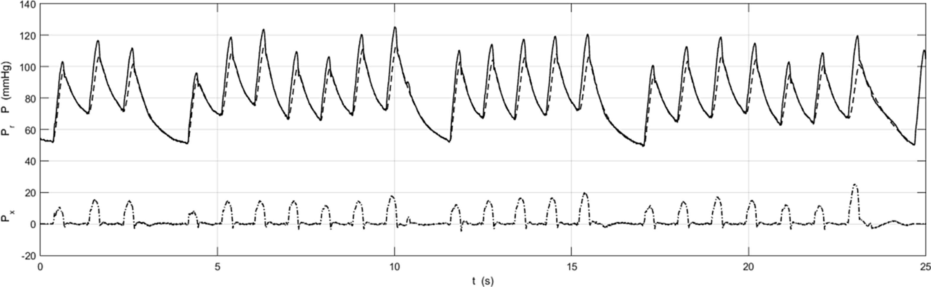
The pressure was measured sequentially at 5 locations in the aorta; 1-the ascending aorta, 2-the transverse aortic arch, 3-the descending aorta at the level of the diaphragm, 4-at the level of the renal arteries and 5-at the aortic bifurcation; by withdrawing the pressure transducer tipped catheter to the appropriate location determined by angiography. The pressure was measured for 25 s at each site, Fig. 2. These data were ensemble averaged by an algorithm that excluded outlier beats automatically (based on the magnitude of the correlation of the beat to the ensemble average beat). The ensemble average waveforms P were used to calculate the reservoir Pr and excess Px pressure using the pressure-only algorithm. Figure 3 shows P − Pd, Pr − Pd and Px at the 5 measurement sites in one of the patients, where Pd is the diastolic (minimum) pressure measured at each site, The thin black line connects the diastolic points at the different locations and its slope in the x − t plane is an indication of the wave speed in the aorta.
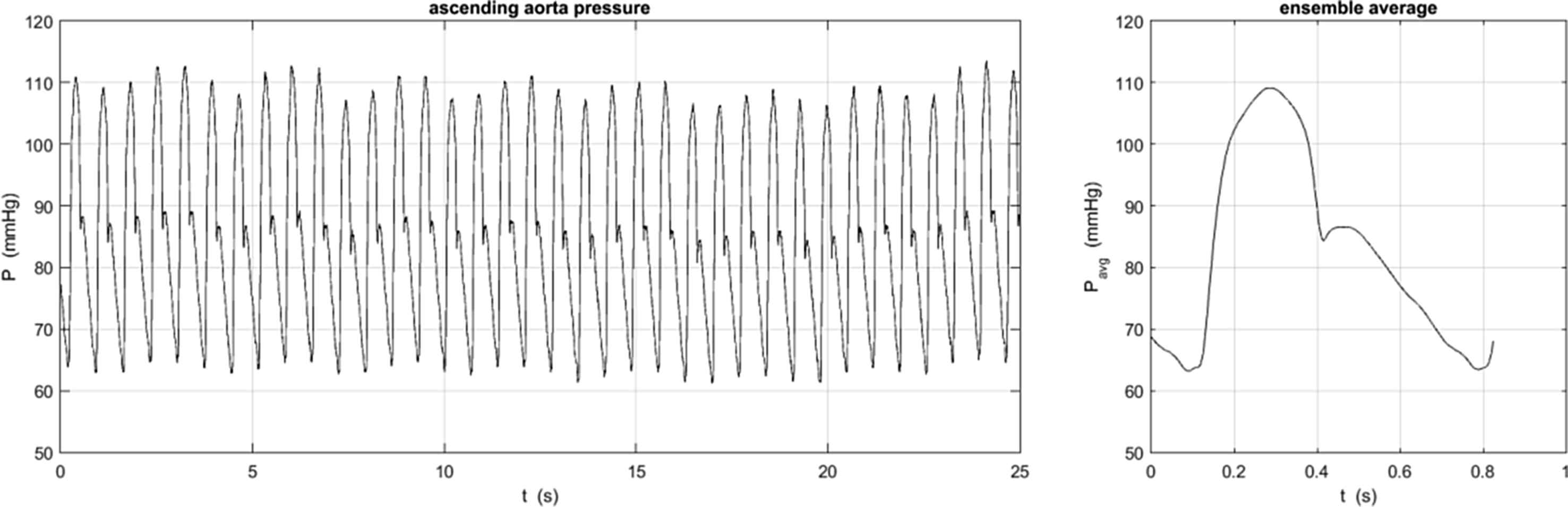
The pressure measured over 25 s in the ascending aorta of one patient (left) was ensemble averaged to give the measured pressure waveform used in the analysis. The standard deviation at each measurement time is not shown but was generally of the order of 4 mmHg, mainly due to the respiratory variation in the pressure seen in the measured data on the left. Some patients exhibited missing or ectopic beats and these were ignored in the calculation of the ensemble average pressure waveform.
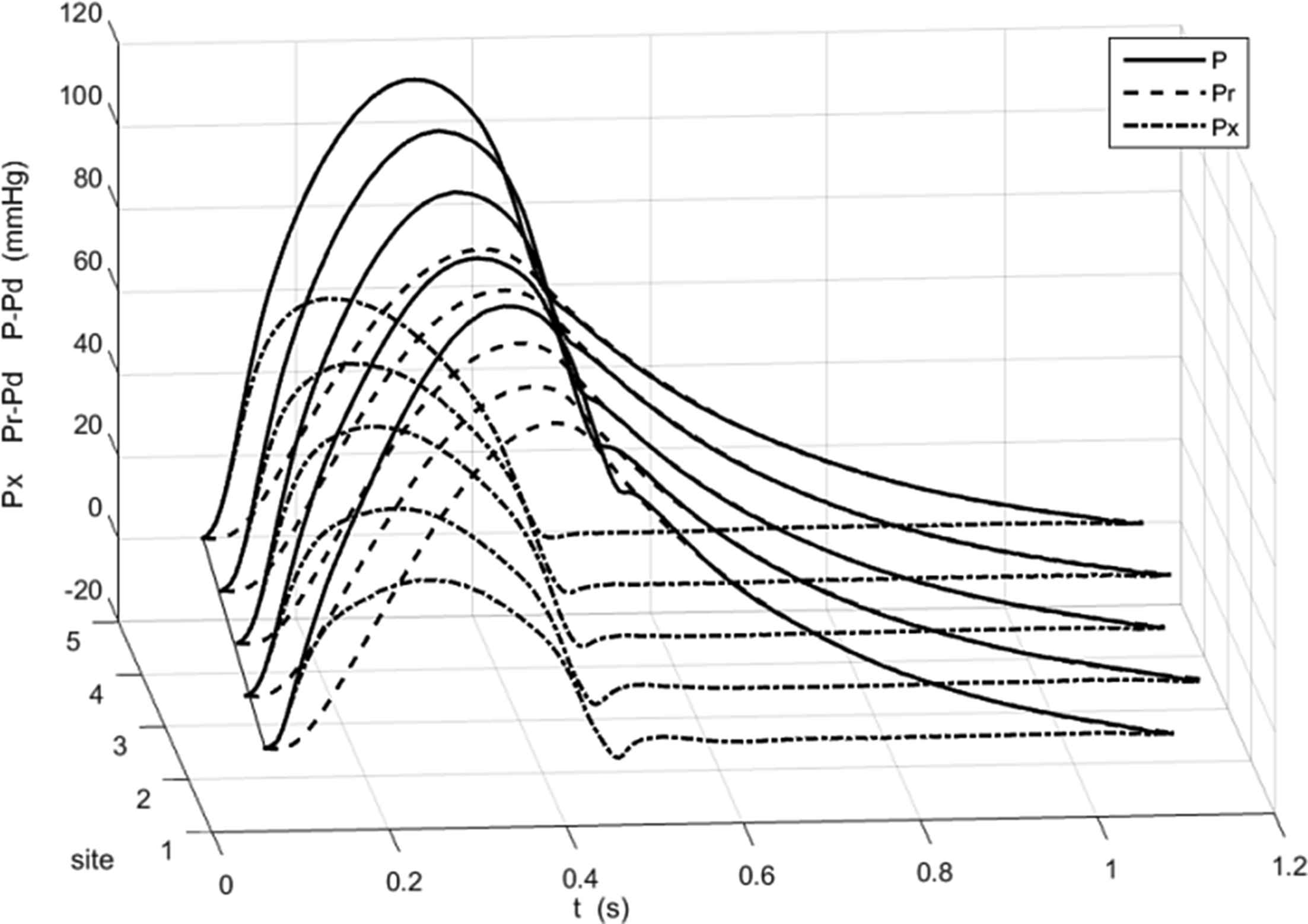
The ensemble average pressure P − Pd (solid line), the calculated reservoir pressure Pr − Pd (dashed line) and excess pressure Px (dash dot line) at the 5 measurement sites in one of the patients. Pd is the diastolic pressure. Since the measurement sites were determined by angiography they are indicated by their index rather than a distance along the aorta.
There are several notable features of this plot, which are common to all of our measurements. First, in all cases,
Pr is very close to P during diastole. This is not surprising because the algorithm that calculates Pr derives two of the fitting parameters by fitting an exponential model to the diastolic portion of P. Second, Px is very close to P during very early systole. This follows from the model of Pr as a solution of the equation for overall mass conservation in the arteries
These observations were tested by applying intra-class correlation analysis to the data at all of the sites in all of the patients. The results shown in Fig. 4 confirm the conclusions drawn from the results for a single patient shown in Fig. 3. The systolic pressure Ps is shown by the black squares and the black dots indicate the 95% CI in the mean at each site. Mean Ps increases from 135.7 mmHg at the aortic root to 144.3 mmHg at the aortic bifurcation. The peak of

The results of the ICC analysis of patient data at the different sites of measurement: 1-asc aorta, 2-transverse aortic arch 3-desc aorta at the level of the diaphragm, 4-desc aorta at the level of the renal arteries and 5-aortic bifurcation. The solid symbols indicate the mean values and the smaller dots indicate the 95% confidence intervals. (squares, solid line) systolic pressure, (circles, dashed line) peak reservoir pressure and (diamonds, dash dot line) peak excess pressure.
We studied the variation of many other parameters describing the reservoir and excess pressures calculated from the clinical measurements of aortic pressure at different sites in the aorta and anyone who is interested should refer to the paper when it is published. For the purposes of this talk, these measured results support the assumption that Pr is uniform along the aorta. Unfortunately, the flow at the aortic root was not measured and so we could not test the second basic assumption of the pressure-only calculation of Pr that the Px waveform is proportional to Qin in man.
To conclude this section of the talk, we note that the definition of reservoir pressure does not rely on periodicity of the aortic pressure. This is in contradistinction to impedance analysis of aortic pressure where periodicity is implicit in the calculation of the Fourier components of the waveform. For this reason, the results of impedance analysis cannot be extended to unsteady phenomena.
Figure 5 shows the instantaneous P, Pr and Px calculated beat by beat for measurements made in the ascending aorta of one patient exhibiting regular cardiac behaviour. There are variations in the beat by beat measurements of P (solid line) that are most likely due to respiration. Pr (dashed line) and Px (dash dot line) calculated beat by beat also show some variation from beat to beat. We have also calculated the ensemble average of the beat by beat Pr and Px and find that they are almost identical to the Pr and Px calculated from the ensemble average P.
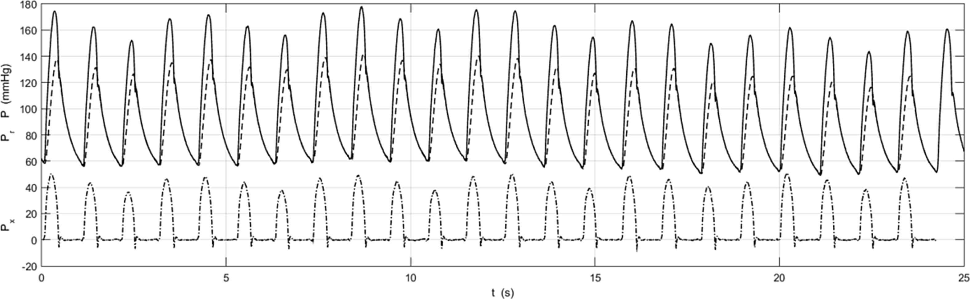
The instantaneous aortic pressure P (solid line), and Pr (dashed line) and Px (dash dot line) calculated from P beat by beat during the 25 s measurement in the ascending aorta of a patient with a regular cardiac cycle. There are variations from beat to beat, probably due to respiration. These difference may be clearer in Px where the peak values vary in a very regular way at a frequency that is commensurate with the (unmeasured) respiratory cycle.
Figure 6 shows the pressure measurements in the ascending aorta of a patient who exhibited a number of long beats during the period of measurement. The main message of this plot is that it is possible to calculate Pr and Px during highly irregular cardiac behaviour. We have not explored the utility of this separation but it seems likely that the excellent fit of Pr to P during extended diastole is telling us something about arterial mechanics during irregular beats and that this mode of analysis my be useful in developing a better understanding of arterial mechanics during these periods.
P, Pr and Px (format identical to Figure 5) for a patient with a highly irregular cardiac cycle. Note that it is possible to calculate Pr and Px during both the ‘normal’ and ‘extended’ cardiac cycles. The ability to analyse irregular beats suggests that this mode of analysis may be useful for studying patients who are not exhibiting regular cardiac behaviour.
To summarise this section, we have shown:
- (1)
Pressure has been defined and divided in many ways, some useful, some not.
- (2)
Reservoir and excess pressure can be calculated from pressure measurements in the human aorta.
- (3)
Reservoir pressure propagates down the aorta at the same speed at the measured pressure waveform.
- (4)
Reservoir pressure is not non-uniform down the aorta.
- (5)
Reservoir and excess pressure can be calculated in irregular beats and may be helpful in understanding these unsteady phenomena.
Low-frequency arterial pressure waves
In part 2 of my talk I would like to describe an asymptotic analysis of the input impedance of a simplified arterial tree. Those of you who know my previous work on wave intensity analysis may be surprised at this direction in my research. I am not well-versed in impedance analysis and the presence in the audience of Nico Westerhof and Michael O’Rourke, both founders and proponents of the subject, is a bit daunting. It may also appear that this part of my talk is outside of my assigned title, but I hope to convince you that there is a connection. In fact, the starting point of this work is my belief that both impedance and wave intensity analysis are founded on the same mechanical principles and therefore they should share many similarities.
The stimulus for this study is a paper published by M.G. Talylor in 1966 where he calculated the input impedance of a highly idealised arterial network (uniform bifurcating tree with 7 generations) with identical properties except that the vessels in each generation had randomly generated lengths.11 In a heroic calculation, given the primitive nature of computers at the time, he generated different random networks and calculated their input impedances which he presented as power spectra. He published the results for 3 different realisations shown in the insets in Fig. 7.
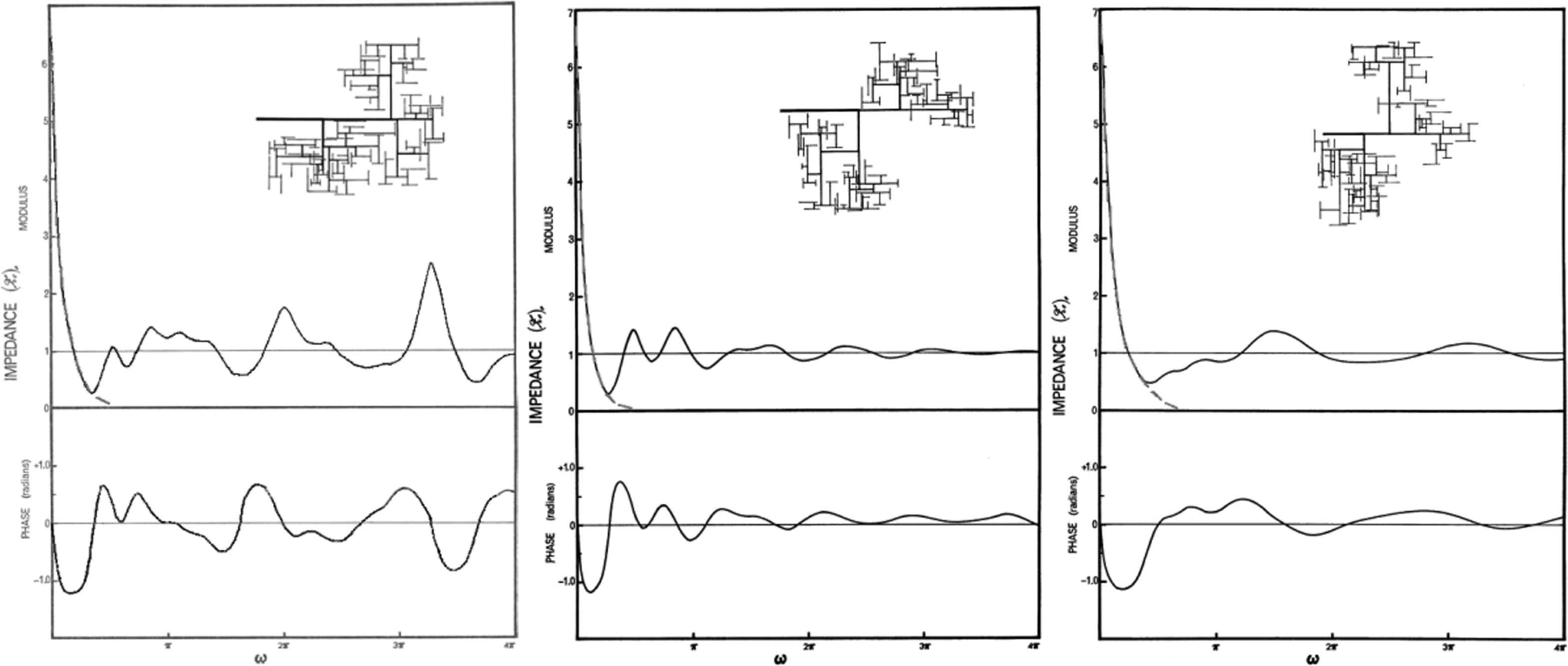
The power spectrum of the input impedance calculated for the randomly generated arterial trees shown in the insets.11 All of the properties of the vessels making up each generation were uniform except for their randomly generated length. The terminal impedances of the terminal branches (seventh generation) are identical for every case. The black lines are copied from Figures 6–8 from the paper with other lines giving results for different values of the terminal resistances removed. The grey dashed line is a fit to the low-frequency input impedance suggested by the analysis. It is not part of Taylor’s results.
The most striking thing about these results is how different the input impedances are from each other over the range of frequencies calculated. The only feature of the spectra that is constant in these randomly generated networks is the low-frequency behaviour,
Asymptotic analysis of the input impedance
For the analysis I assume that the arterial network is a bifurcating tree (not necessarily a symmetrical tree) where all of the properties of the individual arteries are uniform and known: length L, area A, compliance C, wave speed c, wave travel time T and characteristic impedance z. The nodes in the tree are assumed to be bifurcations (internal nodes) where three vessels connect or termini (external nodes) where the terminal arteries are connected to simple known resistances and the root is connected to the ventricle.
We assume that the wave speed c in each vessel is real and given by the Bramwell–Hill relationship
The asymptotic analysis is based on the equations derived by Westerhof relating the impedance Z0in at the input of vessel n to the reflection coefficient Γn at the terminal end of the vessel.12
Since trees are parallel in their structure, it is most convenient to recast these equations into terms of admittances Y = 1/Z.
To complete the analytical formulation for a bifurcating network, Westerhof showed that the outlet admittance of the parent vessel is equal to the sum of the input admittances of the daughter vessels (Kirchoff’s law).
If we define the maximum wave travel time over all of the vessels in the tree
T = max(Tn) and
If we assume that the admittances have the form Y = σ + iωTη where σ and η are real, we can derive the asymptotic recursion relations
I have not been able to think of a simple physical explanation for the form of this effective, weighted compliance, but there is a simple argument that indicates the need for some form of weighting. Consider a terminal vessel whose characteristic impedance matches its terminal resistance. The reflection coefficient at the terminal end of this vessel will be zero (Snzn = 1) and so the wave in this vessel will not be reflected back into the rest of the tree. This means that the rest of the network is not influenced by the compliance of that vessel and we would not expect it to affect the first order behaviour of the tree. The weighting
Reverting to impedance, these results indicate that the low-frequency behaviour of the tree is
This is familiar as the input impedance of a 2-element Windkessel with net arterial resistance R and compliance equal to the effective compliance
Low-frequency flow and pressure
Having derived the low-frequency input impedance of the arterial tree, we can now calculate the pressure and flow throughout the network starting at the root and working downward through the tree. We first observe that flow in the parent vessel (index a) at a bifurcation distributes into the daughter vessels (indices b & c) depending on their input impedances.
Substituting the low-frequency admittances
By definition of admittance,
The summation in this expression is simply the summation of the effective wave travel times over all of the vessels on the path from the root of the arterial system to vessel n. Using the bar notation for net quantities previously used for
We conclude this section by noting that the low-frequency component of the pressure shares the fundamental properties of the reservoir pressure, it is uniform throughout the arterial system but delayed by a wave travel time. In the present company I am reticent to claim that it is the reservoir pressure; this will require further analysis and study. However it is clear, whatever your biases about impedance and wave intensity analysis, that the low-frequency component of the pressure has some interesting properties and certainly warrants further study.
To summarise this section, we have shown:
- (1)
The low-frequency input impedance is Windkessel-like:
- (2)
The relevant compliance is an effective compliance:
- (3)
The low-frequency pressure is uniform throughout the arterial system, but delayed by a wave travel time:
- (4)
The wave travel time is the effective wave travel time:
Arterial mechanics via wave fronts
The third part of my talk is inspired by ‘future’ in the title of this meeting and concerns my current work using wave fronts to analyse arterial hemodynamics. The work has progressed since I gave the talk and this section is based on my most recent results. These differ in some technical aspects from the work that I described in my talk, but the broad (and tentative) results remain the same.
The spirit of the analysis is to explore the influence of the complexity of the arterial network on its hemodynamics by constructing a model that minimises the many other complexities of arterial mechanics. To do this we assume that the arterial system can be modelled by a network of uniform arterial segments connected together at bifurcations and connected to the heart at the root. We assume that flow in the individual arteries can be described by the 1-D conservation equations of mass and momentum. We neglect viscous dissipation in the arteries and viscoelastic effects in the arterial walls. We further assume that the terminal vessels in the network are connected to the venous system by simple resistances describing flow through the microcirculation. In our latest work we consider the possibility of networks with loops so that we can study the effects of anastomoses on arterial hemodynamics.
As a final simplification, we consider what happens to a single wave front introduced at the root at t = 0. This, in fact, is not a limitation of the work because we can analyse more complex input waveforms by convolution of the single wave results. It does, however, greatly simplify the presentation of the results. Physically a single wave front at the root is equivalent to imposing a step change in flow (or pressure) at the root and then looking at the response of the arterial system to that change in conditions.
To help make our results concrete, we will present results based on probably the most widely used arterial model, the 55 artery model introduced by Westerhof14 during his PhD research and later modified by Stergiopulos15 during his PhD research. Amongst many others this model has been used by Segers16 in his experimental PhD research and Alastruey17 in his computational PhD research. I suspect that Nico Westerhof had no idea when he was collecting data for his model that he was producing such an effective PhD-machine. The model is a tree without any loops and is shown in Fig. 8a in a form that emphasises its binary tree structure with 55 edges (arteries) and 56 nodes, 27 internal and 29 external. the altitude of the tree, the maximum number of generations, is 14. A more anatomically recognisable version of the tree is shown in Fig. 8b. Here the length of each edge is approximately proportional to its physical length and the head and neck arteries have been moved from under the right arm to a position above the heart. In a 1-D model, the propagation of waves in an arterial segment depends only on axial distance and does not depend on its spatial geometry. That is, the behaviour of waves in the arteries, in this approximation, depends only on the topological connectivity of the arteries and not their geometry.
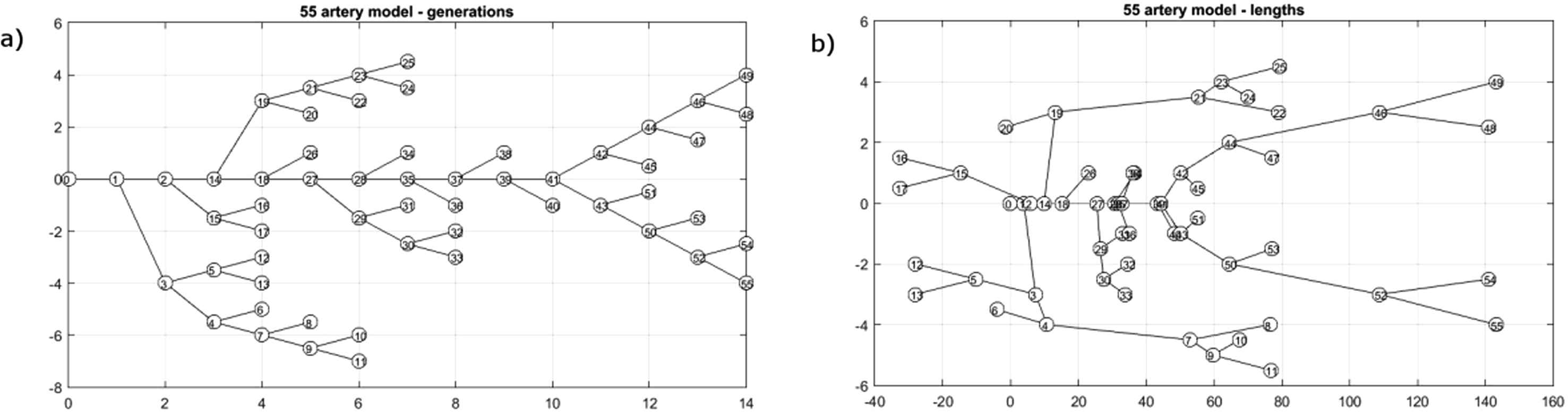
The 55 artery model used for the calculations.13 The binary tree nature of the network is shown in the sketch (a) where the edges (arteries) are arranged by their generation. In the sketch (b) the length of the edges is approximately proportional to their physical length and the head and neck arteries have been moved from below the right arm to above the location of the heart (the root of the tree). It should be more recognisable anatomically although the aorta is shown as straight rather than arched.
The generation and evolution of wave fronts in the arterial tree
The 1-D conservation equations in each vessel together with a suitable tube law describing the change in area of the vessel with pressure give a hyperbolic system of ODEs. They are amenable to solution by the method of characteristics introduced by Riemann.18 The salient feature of this solution for our model which neglects viscous effects is that any perturbation of conditions in the vessel will propagate as a wave in both the forward and backward direction. Following the example of gas dynamics where the 1-D model is well-developed, we will assume that the basic form of wave is a wave front, a step change, either positive or negative, in the pressure and the flow across the wave. It is easy to build any waveform by a sequence of discrete wave fronts which makes them convenient as a basis for any waveform. We make the further simplification that the wave fronts are linear in the sense that they are additive and do not interact with each other when they cross. This assumption is essentially the acoustic limit in fluid dynamics and can be ensured in the absence of shock waves simply by considering wave fronts whose amplitudes are sufficiently small.
With all of the simplifying assumptions we can think of each wave front as a ‘particle’ that propagate unchanged through the edge (vessel) until it encounter a node. When it encounters an external node the wave front is reflected with a magnitude that is given by a reflection coefficient. When it encounters an internal node the wave front produces three wave fronts, a reflected wave front with a magnitude given by a reflection coefficient and two transmitted waves with magnitudes given by a transmission coefficient. The problem thus reduces to following the evolution of the single wave front introduced at the root at t = 0.
Because the interaction of a wave front with an internal node produces three waves, the total number of waves in the system will grow exponentially. The amplitude of the new waves decreases on average and we will see that the amplitude gets exponentially small as the number of waves gets exponentially large. The net effect of the myriad numbers of vanishing small waves is not immediately apparent and we have to be careful in the analysis not to truncate results inappropriately.
To facilitate the tracking of the waves in the system we introduce the idea of a wave history Wn = {e0,e1,e2, …,ei,ei+1,…,eN−1,eN} which is the sequence of edges visited by wave n. For waves introduced at the root, e0 = 1. N is the number of edges visited by the wave which leads to the concept of a step, which is defined as going from one node of the edge to the other. Because each edge has a wave travel time associated with it, the time it takes a wave to execute one step depends upon the vessel it is in. This leads to difficulties in calculating the location of a wave at a particular time whereas locating a wave after a given number of steps is simple. The synchronisation of steps with time is a final step in the analysis.
After N steps the total time (duration) of wave Tn is the sum of all of the wave travel times in all of the edges it has traversed
The amplitude of the wave An is the product of all of the reflection and transmission coefficients at all of the nodes it has encountered
The exponential growth of the number of wave fronts and hence wave histories is an important feature of this theory. The exact number depends on the topology of the network. For large N the number of waves is given by the recursion formula
Fortunately the importance of large networks on modern life has stimulated many advances in the field of network theory and we will adopt some of these methods into our analysis. Networks can be described in many ways but for our purposes the most convenient representation is the connectivity matrix. For a network with N nodes and E edges the connectivity matrix is an N × E matrix with each row representing one node and each column representing one vessel (edge). By definition each edge is connected to 2 nodes, one identified as the input node and the other the output node. In rooted binary trees, it is straightforward to describe the node closest to the root as the input node. In more general networks with loops, this is not possible and the designation of input and output nodes can be arbitrary. Each column in the connectivity matrix has −1 in the row of the input node and +1 in the row of the output node. All other entries in the row are zero. This matrix provides a complete description of the topology of the network. In particular summing the number of non-zero entries along a row gives the degree of the node defined as the number of edges that are connected at that node. We assume that the arterial network can be modelled by nodes of degree 3 (internal bifurcations) or of degree 1 (external nodes). Real arterial networks sometimes include trifurcations but these are rare and it is almost always possible to model them as two bifurcations separated by a very short edge.
Given the topology of the network, it is necessary to find a compact way to represent the reflection and transmission coefficients at the nodes. For an external node k connecting a resistance Rk to an edge with a characteristic impedance zk, the reflection coefficient Γk is
This is the same as the reflection coefficient defined in the impedance analysis in Section Reservoir and excess pressure along the human aorta. The reflection and transmission coefficients for an internal node depend upon the edge in which the wave front approaches the node. For an internal node i connecting edges a, b and c the reflection and transmission coefficients are given by the 3 × 3 matrix
Knowing the reflection and transmission coefficients at each node, we can now construct a global matrix of coefficients for the whole network. For a matrix with E edges, this will be a 2E × 2E matrix where each edge has a separate row for the forward and backward waves in the edge. For a large network this can be a rather large matrix, for example the matrix for the 55-artery model is 110 × 110, but the matrices are sparse (mainly zero elements) and they can be easily accommodated by current computers. We term this matrix the ‘scattering matrix’ by analogy to scattering theory in acoustics and microwave transmission theory. Calculating the amplitude of the waves in the system now reduces to a problem of matrix multiplication. Given an initial wave at the root with amplitude a0 =[1,0,0,0,…,0]T, i.e. a unit step wave at the root) the amplitude of the waves in the system after N steps is given by
Thus, the history of the waves in the system after N steps is reduced to evaluating the powers of Γ.
Eigen-modes and time constants
Although computers can calculate the power of a large matrix very quickly, the representation and interpretation of the results is difficult. Fortunately linear algebra provides a way to deal with the problem that provides results that are easy to interpret; eigenvalues and eigenvectors. An eigenvalue λ and eigenvector v of matrix Γ are defined by the equation
That is, multiplying an eigenvector by the matrix results in a scale factor times the eigenvector. This is very convenient when we are taking powers of the matrix because successive multiplications by the matrix yields
Thus, the power of the matrix times an eigenvector is just the power of the scalar eigenvalue times the eigenvector, and the problem of matrix multiplication further reduces to multiplication by a scalar.
Because they are central to matrix calculations, the theory of eigenvalues and eigenvectors is a well-studied branch of linear algebra. In general an N × N non-degenerate matrix can have N eigenvalues each of them with an associated eigenvector. The eigenvalues determined by finding the roots of an N th order polynomial, however, are not necessarily unique and it is difficult to determine the multiplicity of eigenvalues without calculating them. Also, for a real matrix the eigenvalues can be complex in which case they occur as conjugate pairs, and these have complex conjugate pairs of eigenvectors associated with them.
Traditionally the eigenvectors are taken to be unit vectors because it is the direction of the eigenvector, not its amplitude, that is important. Since the sum of the square of the absolute value of the coefficients of a unit vector is equal to 1, the eigenvectors can be thought of as eigen-modes associated with each eigenvalue. The evolution of these eigen-modes as the number of steps in increased is determined by the absolute value of the eigenvalue. If we define Am(N) to be the amplitude of mode m, after N steps then
Physically we are interested in the behaviour of the system with time, not with the number of steps taken by the wave fronts. To relate the results in terms of steps to time forces us to turn to statistical methods. Given the wide range of wave travel times in the arterial network (in the 55 artery model they range from 1.9 ms for the celiac artery to 71.5 ms for the two brachial arteries). Fortunately, we can apply statistical arguments with a high level of confidence, given the large number of waves that are generated.
For our analysis, we assume that the time it takes to execute N steps is given in a probabilistic sense by t = N〈T〉, where 〈T〉 is the appropriate average wave travel time. There are a number of candidates for the appropriate average, but we believe that best choice is the weighted average wave travel time for each particular mode. As discussed previously, this weighting is the square of the magnitude of the coefficients of the eigenvector which defines the mode. That is, for mode m
The minus sign in the definition is usual since we are only interested in eigenvalues with |λ| ≤ 1 with negative logarithms.
The conclusion of this analysis is that the for large times, when we can expect t = N〈T〉 to be a good estimate, each of the modes of the system will contribute an exponentially decaying term with different time constants for each of the modes. The long-time behaviour of the system will depend on the mode with the longest time constants, since the other modes will die away more quickly. Ideally this time constant would correspond to the time constant that is usually cited for the diastolic pressure decay. For the limited number of cases which I have studied, this is not the case and the largest time constants are commonly two or three times larger than the expected diastolic time constant. This could be due to deficiencies in the models I have used, an extraordinary number of parameters is needed to define a realistic arterial network. Alternatively, it could be related to problems associated with fitting a single exponential to a multi-exponential function.
Results for the 55 artery model
The above analysis is abstruse and undoubtedly difficult to follow without a background in large dynamical systems. I will try to make the important points clearer by presenting the results of this analysis applied to the 55 artery model of the human circulation. This model has been used extensively in model calculations and I have based my work on a slightly simplified version of the model used by Alastruey and his colleagues in their numerical computations (refer to Ref.13 for an example of their work). The main simplifications are the assumption of uniform arteries (no taper) and real terminal impedances (resistances with no compliance). With these assumptions it is possible to calculate the characteristic impedance of each vessel and, knowing the connectivity of the network, the reflection and transmission coefficients at all of the nodes. These were used to construct the 110 × 110 scattering matrix Γ.
The eigenvalues and eigenvectors of Γ were calculated using MatLab. The level of multiplicity of the eigenvalues was fairly large and there were only 30 unique absolute values of the eigenvalues. The eigenvectors associated with each of the unique eigenvalues defined 30 different modes for the network. Table 1 shows the time constant τ in s, the magnitude of the eigenvalue |λ | and the mean wave travel time 〈T 〉 for the modes with the 6 largest time constants and for the mode with the smallest time constant, ranked according to the time constant.
| τ (s) | |λ| | 〈T〉 (ms) |
|---|---|---|
| 1.78 | 0.961 | 71.5 |
| 1.18 | 0.972 | 33.4 |
| 1.14 | 0.939 | 71.5 |
| 0.98 | 0.961 | 39.2 |
| 0.88 | 0.989 | 9.3 |
| 0.70 | 0.965 | 24.7 |
| ⋮ | ⋮ | ⋮ |
| 0.08 | 0.01 | 2.2 |
The magnitude of the time constants, the eigenvalues and the mean wave travel times for 7 of the 30 distinct modes of the 55 artery model arranged in descending order of the time constants. The modes for the 6 largest time constants are shown in Fig. 9.
Representations of the modes is difficult because the indices of the arteries in the model are somewhat arbitrary (see Fig. 8). We show them graphically in Fig. 9 where the grey level of each artery is an indication of its weight in the mode. The mode with the largest time constant (upper left) is dominated by the arteries in the arm. The magnitude of the eigenvalue for this mode is only the 4th largest but the largest wave travel time is for the brachial artery and this is reflected in the time constant for the mode. The modes with the next 3 largest time constants are dominated by the legs and lower arms. The mode with the 5th largest time constant corresponds to the mode with the most uniform distribution of arteries. The smallest time constant (not shown) is interesting because it is almost completely dominated by the celiac artery which has the smallest wave travel time in the model.
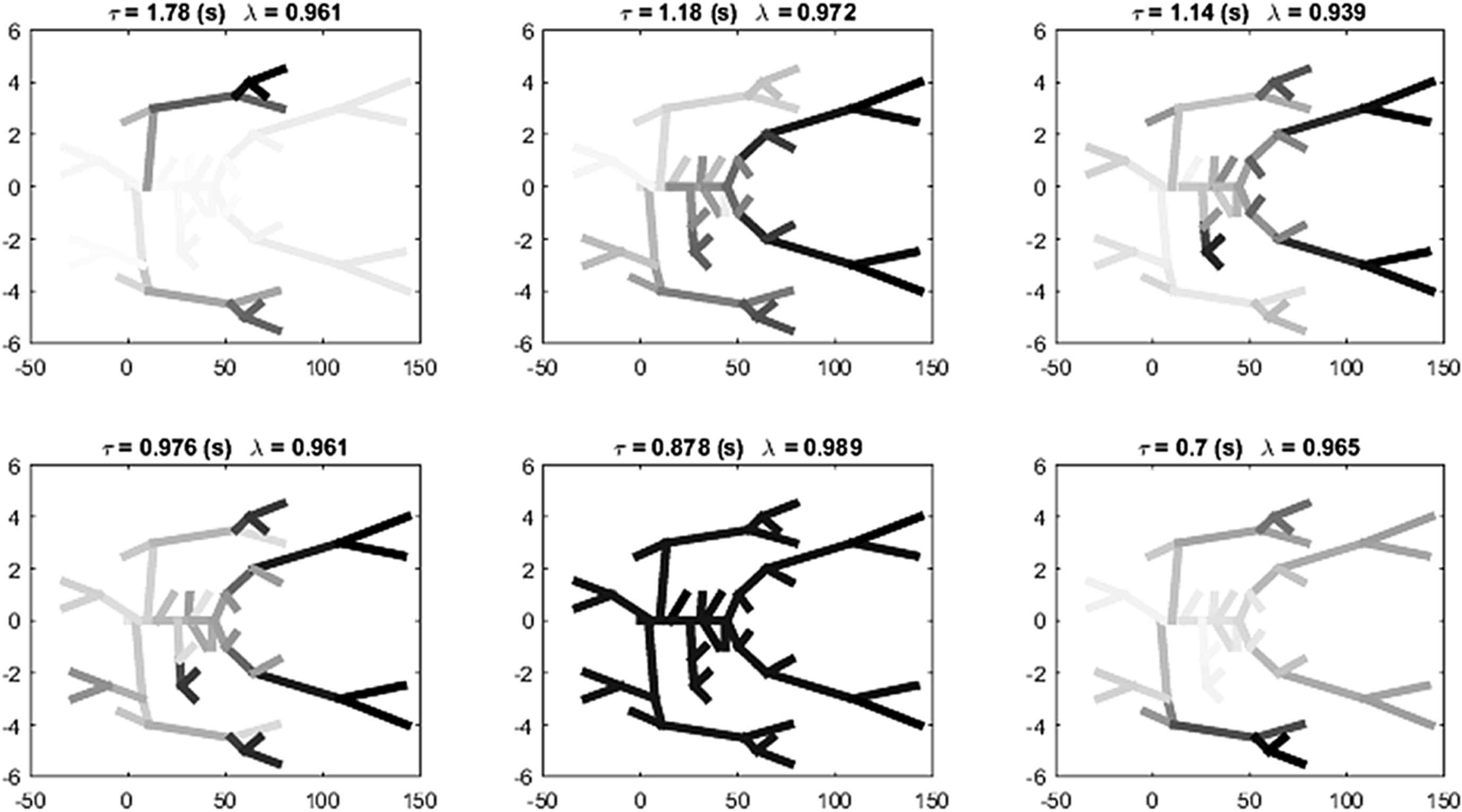
The eigen-modes corresponding to the 6 largest time constants. The grey scale of each artery is an indication of its contribution to the mode.
Implications for clinical measurements of arterial pressure
These results for the evolution of a wave front introduced at the root of the arterial network show that the input wave front will excite a large number of modes in the network which decay with different time constants. Calculating these modes and their time constants requires full knowledge about the connectivity and physical properties of all of the arteries in the network – god-like knowledge that is not available to the clinician. We have to conclude, therefore, that the theory does not offer direct information about the measured waveform. It does, however, offer insights into the physical processes involved which can increase our understanding of the interaction of the heart and the arteries.
The theory indicates that there are many modes that will be stimulated by waves generated by the heart and, after sufficient time, they will decay exponentially with different time constants. Fitting measured data to a multi-exponential function is “notoriously difficult”.20,21 This means that it is very difficult to determine the multiple time constants from measurements of the diastolic pressure decay because there are many combinations of coefficients and time constants that can fit the same data over the limited span of diastole.
This difficulty is illustrated in Fig. 10 where we have fit the decaying pressure during a single diastolic period to (dashed line) a single exponential model with a zero asymptote, (dash dot line) a single exponential model with a free asymptote and (dotted line) a double exponential model with a zero asymptote. The fit of the single exponential without an asymptote (R2 = 0.9663) is significantly worse than the fit of the other models which have identical R2 values (R2 = 0.9995) but the time constant (τ = 0.68s) is closer to the textbook value of the diastolic time constant. The single exponential model with a free asymptote gives a significantly shorter time constant (τ = 0.28s) but a surprisingly high value of the asymptote. The asymptote of the double exponential model is zero but the largest time constant (τ = 5.58s) means that this asymptote is reached very slowly. The smaller time constant for the double exponential model (τ = 0.24s) is close to the time constant for the single exponential with an asymptote model. Fitting higher order exponential models to the data do not lead to any significant increase in the fitting statistics and the results are unpredictable and generally uninterpretable.
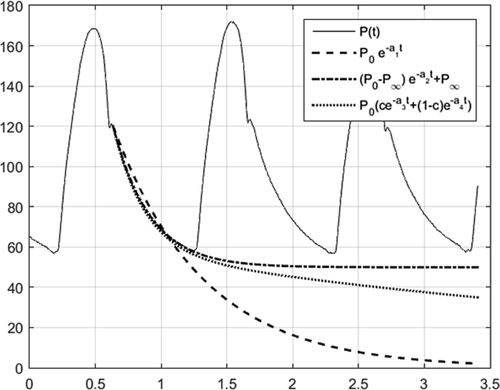
Comparison of different exponential models to the diastolic pressure measured in the ascending aorta. (solid line) P measured for 3 beats in the ascending aorta using an invasive pressure catheter calibrated to atmospheric pressure. (dashed line) data fitted by a single exponential with zero asymptote P = P0e−t/τ1. (dot dash line) data fitted by a single exponential with a free asymptote P =(P0−P∞)e−t/τ2+P∞. (dotted line) data fitted by a double exponential with zero asymptote P=P0(αe−t/τ3+(1−α)e−t/τ4). The single exponent with zero asymptote does not fit the data during diastole as well as the other models. The fits using the single exponential model with asymptote and the double exponential model with zero asymptote are statistically indistinguishable (R2=0.9995 for both cases) but diverge significantly for times longer than the diastolic period. The fitted time constants are τ1=0.68s, τ2=0.28s, τ3=0.24s and τ4=5.58s.
The only message we can draw from this example is that there are many exponential models that will fit the decaying diastolic pressure. The fitted time constants depend on the choice of model and so it is probably wrong to cite the time constant as a unique parameter describing diastole. The second message is that using any of the models fitted during the diastolic period can be used with confidence during diastole but should be used with caution when extrapolating to longer times.
The implications of this to the determination of the reservoir pressure which involves fitting the diastolic pressure with a single exponential with a free asymptote and extrapolating this into the systolic period are uncertain and warrant further research. The work described here suggests that the reservoir pressure should have a multi-exponential form but the uncertainty in fitting such a model to diastole limits the practical usefulness of this result. It is clear, however, that the long-time effect of the wave fronts generated by the input from the heart to the arteries is not negligible. This can be illustrated very clearly by looking at some computational results for the simplified 55 artery model (kindly generated by J. Alastruey) where the pressure in the ascending aorta was calculated for a given periodic flow from the heart. The calculations were started at arbitrary initial conditions and continued until the calculated pressure became periodic, at which point the input from the heart was stopped, corresponding to an indefinitely extended diastole. The result of that calculation is shown in Fig. 11.
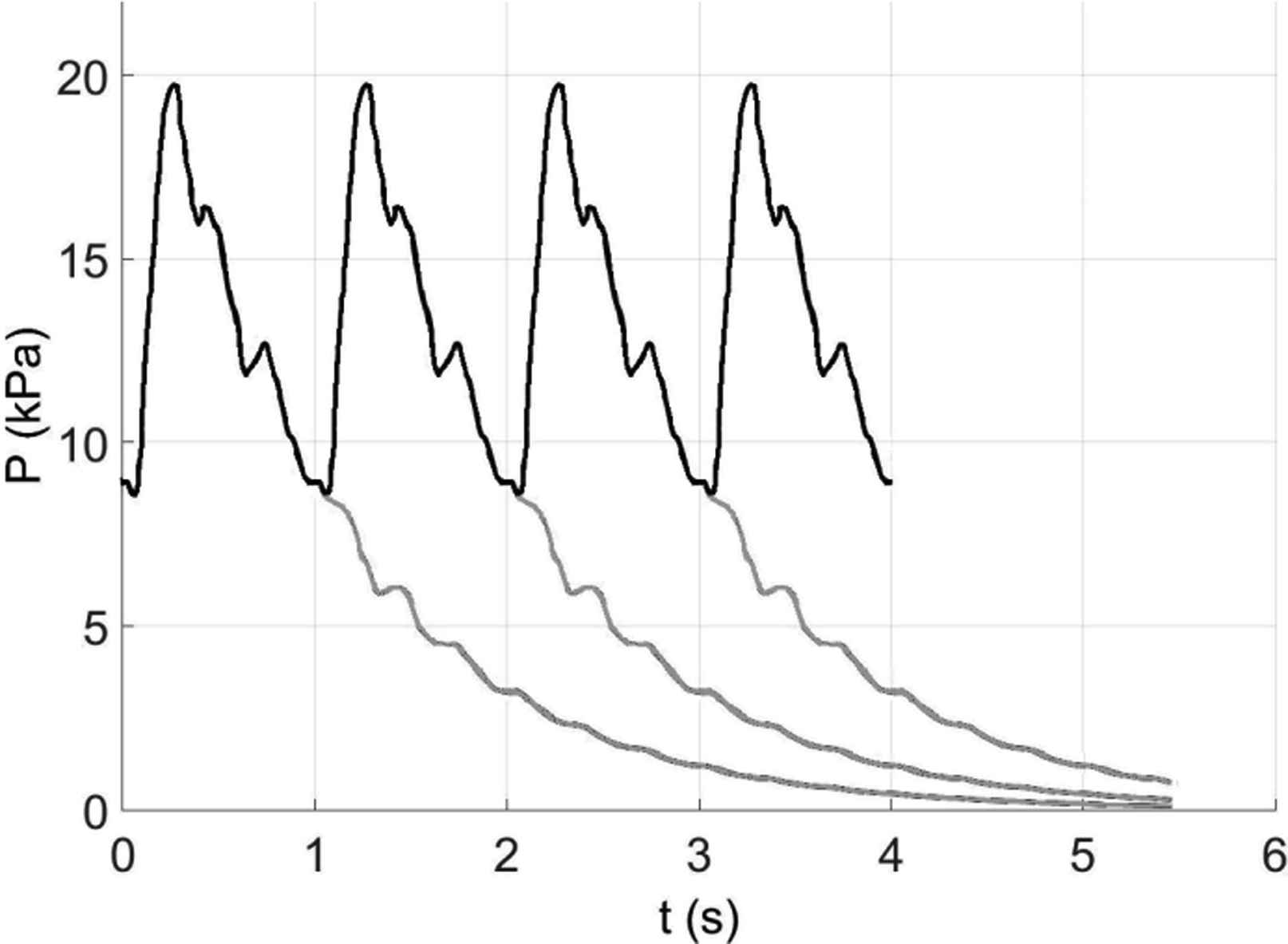
The pressure in the ascending aorta calculated by J. Alastruey for the simplified 55-artery model used in this study. The black line shows the periodic pressure that is generated by a given periodic inflow from the heart. Note that the relatively large fluctuations in pressure seen in late systole and mid-diastole and persist for at least 2 s into the extended diastole do not appear in his calculations which include a significant level of compliance the terminal impedances in the model. The grey lines are the results obtained when the input from the heart was stopped to model the effect of an extended diastole. Because the pressure was periodic, with a period of 1 s, the light grey lines show the pressure that would result if inflow from the heart was stopped after 1, 2 and 3 beats. Looking at the fourth beat in the sequence, we see that nearly half of the diastolic pressure (the minimum pressure at the start of the next systole) is due to the pressure that would be present in the artery if the inflow was stopped at the end of the second beat. Furthermore, about half of that pressure is due to the pressure remaining in the arterial system due to the first beat. This exponentially decreasing contribution from previous beats further and further away from the current beat is typical of exponential processes and is clearly not negligible. It is this contribution to the arterial pressure that is modelled by the reservoir pressure.
The light grey lines indicate the pressure in the ascending aorta calculated assuming that the flow from the heart into the arteries was stopped before the start of the next systole. Because the calculated pressures are periodic, we can plot the result of extended diastole occurring after first, second or third beat. In this way we can see the effect of the previous systoles on subsequent beats. In this example, approximately half of the diastolic pressure at the start of a beat is due to pressure that was generated by the previous systole. The pressure due to the systole two beats before the current beat contributes about a quarter of the diastolic pressure and this contribution falls of exponentially with all of the previous beats. For this calculation we know that the pressure will asymptote to zero and fitting a single exponential model with a zero asymptote give a time constant to the extended diastole τ = 1.02s. Looking at Table 1 we see that this fitted time constant is in the middle of the 6 largest time constants calculated for the this model. This suggests that the calculated data could be fitted equally well with a single exponential model or a high order exponential model with time constants given by the theory.
Conclusions
To conclude this part, we must emphasise that this method of analysis of arterial hemodynamics is new. It is work in progress and the results should be considered to be preliminary. Although we have made many simplifications in the analysis presented here, these simplifications are not essential to the approach and most of them can be relaxed at the cost of more complex analysis. In particular looking at the case of a single wave front introduced at the aortic root at time zero does not limit the generality of the analysis since any waveform at the root can be decomposed into a sequence of individual wave fronts and the results for the general case can be found by convolution of the single wave front results.
The initial aim of the work was to provide a theoretical basis for the reservoir-wave hypothesis but that has not yet been achieved. Another aim was to explore the effect of the complex anatomy of the arterial network, a binary tree with a large number of edges (vessels) including a number of loops (anastomoses). To explore this question we considered a highly simplified model (inviscid, uniform arteries, etc.) where the only source of complexity was the morphology of the arterial network. The results indicate that the reflection and re-reflection of the single inputed wave front generates complexity that increases exponentially with time. These results support the argument that simple single-vessel or T-tube modes of the arteries can give misleading results.22
The idea of a wave history, the list of all the vessels traversed by a particular wave front, with the ancillary concept of a step, the traversal of one vessel, provides a systematic approach to the exponentially growing complexity. For short times this approach could yield a detailed description of arterial hemodynamics. As time increases the number of wave fronts increases to the point where the combinatorial complexity of their wave histories will make detailed analysis impossible on even the largest computers.
Fortunately, as the number of waves increases their statistical analysis becomes increasingly valid and accurate. A crucial point in this analysis is that the number of steps in the history of a wave N can be related to the time statistically; t = N 〈 T〉 where 〈T〉 is an appropriate average wave travel time. Because the wave travel time varies greatly between the vessels, the time taken to execute N steps will vary greatly for short times. For longer times the paths of the different waves will start to overlap and eventually all of the wave fronts will have, on average, visited the whole arterial network in different sequences. The results we have presented pertain to these old waves and my current belief is that the reservoir pressure is the sum of the ‘old’ waves and the excess pressure is the sum of the ‘new’ waves. This is, of course, an intuitive rather than a rigorous statement.
Figure 11 suggests that the old waves, which we have shown decay exponentially with time, dominate diastole. Furthermore by extrapolating this behaviour through the next systole (the old waves are not turned off by the start of a new systole) we see that the diastolic arterial pressure can be seen as the summation of the old waves generated by all of the succeeding systoles.
None of the results presented here suggest new measurements or analyses that will be immediately useful in the clinic. My clinical colleagues, normally so receptive and helpful, would tell me to get lost (very politely) if I asked them to measure the geometry and wave speeds of all of a patient’s arteries so that I could calculate their eigen-modes. However, I believe that this new way of looking at arterial hemodynamics will lead to a deeper understanding and, eventually, to improved clinical methods.
To summarise this final section, we have shown:
- (1)
The evolution of a single wave front at the root of the arterial system at t = 0 can be calculated from the scattering matrix describing the reflection and transmission coefficients in all of the arteries.
- (2)
The eigenvalues and eigenvectors of this matrix define a large number of eigen-modes.
- (3)
Each eigen-mode decays with a different time constant.
- (4)
In a 55 artery model, up to 30 eigen-modes exist with different time constants.
- (5)
Testing the theory is difficult because of the difficulty in fitting multi-exponential models to data.
Conflict of interests
The author has no conflict of interests in presenting this work.
Footnotes
It has been asserted that the reservoir pressure is simply 2 times the backward pressure waveform discussed previously.6 This assertion is based on the following (paraphrased) argument: In deriving Pr from P it is assumed that Px ≡ P−Pr = zQ where z is the characteristic impedance. Rearranging, Pr= P − zQ. The backward pressure waveform is derived using
J. Mynard pointed out to me after the talk that this number is equal to the estimated number of atoms in the universe.19 Intuitively I felt that the calculation leading to this result must be flawed but it is, in fact, consistent with the exponential growth of complexity. For example, Shannon, the founder of information theory, estimated a lower bound for the possible number of moves in chess to be 10120.
References
Cite this article
TY  - JOUR
AU  - Kim H. Parker
PY  - 2017
DA  - 2017/04/26
TI  - The reservoir-wave model☆
JO  - Artery Research
SP  - 87
EP  - 101
VL  - 18
IS  - C
SN  - 1876-4401
UR  - https://doi.org/10.1016/j.artres.2017.04.003
DO  - 10.1016/j.artres.2017.04.003
ID  - Parker2017
ER  -